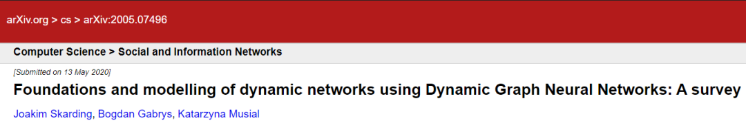
Graph neural networks (GNNs) have been widely applied to the modeling and representation learning of graph-structured data. However, mainstream research has been limited to handling static network data, while real complex networks often undergo structural and property evolution over time. The team led by Katarzyna at the University of Technology Sydney recently published a preprint paper that classifies actual complex networks based on time scales and summarizes various graph neural network architectures used to represent dynamic complex network data.
This article was first published by the Intelligent Graph Club. For the complete list of paper materials, please scan the QR code to obtain:

Dynamic network models add a temporal dimension to static networks, enabling them to represent both the structure and temporal information of complex systems. They are widely used in fields such as biology, medicine, and social networks. Moreover, while GNNs have made significant strides in data mining of static complex networks, most work cannot handle this additional temporal dimension. Considering that real networks are mostly time-varying complex networks, the dynamic graph neural network (DGNN) architecture will undoubtedly be an important research direction. A recent review systematically summarizes the achievements in this field and can be used to understand this emerging research direction.
The authors of this review are the Katarzyna Musial-Gabrys team from the University of Technology Sydney (UTC). Katarzyna focuses on the dynamic and evolutionary analysis of complex networks and the modeling of network structures and properties. Recently, her team has concentrated on using machine learning and predictive models to study dynamic complex networks.
This review can be divided into the following sections:
-
Classification and representation of dynamic networks;
-
DGNN as dynamic network encoders;
-
Decoding and structural prediction of dynamic network representations: taking link prediction as an example.
1. Classification and Representation of Dynamic Networks
The difference between dynamic (Dynamic) networks and static (Static) networks lies in that the former has: 1) dynamic structures where edges and nodes appear/disappear over time, and 2) dynamic attributes where the states of nodes and edges change over time. This article only considers dynamic networks with dynamic structures. This subsection distinguishes and discusses dynamic networks based on time scales and introduces the discrete and continuous representation methods of dynamic networks.
1.1 Classification of Dynamic Networks
The dynamic changes in the structure of networks are reflected in the appearance and disappearance of edges and nodes. The different durations of these changes determine the properties of dynamic networks. For example, new edges in an email network (mutual emails) appear and disappear instantaneously, while edges in a citation network (mutual citations) never disappear once they appear. By classifying dynamic networks based on the duration of edge appearance to disappearance, we can distinguish the evolutionary mechanisms of dynamic networks.
First, consider the duration of edge appearance to disappearance. According to the duration of edges, dynamic networks can be divided into four categories as shown in Figure 4:
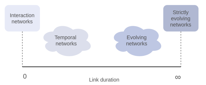
Figure 1: The horizontal axis represents the duration of edges in dynamic networks, allowing the classification of dynamic networks into four categories.
Among them, interaction networks (Interaction networks) and strictly evolving networks (Strictly evolving networks) correspond to the examples of email and citation networks, respectively, representing the two extremes of edge duration: instant disappearance after appearance or permanent persistence. These two cases are relatively easy to distinguish and will not be discussed further in the upcoming classifications.
However, for dynamic networks in the middle of the time axis, the distinction becomes more subtle. The edges in these dynamic networks all disappear after a limited duration following their appearance. Based on this “limited time,” we can classify them into temporal (Temporal) and evolving (Evolving) networks.
Temporal networks have highly dynamic edges with very short durations, making it difficult to sample a complete network structure at any given moment. For example, in interpersonal networks, defining the start and end of conversations as the appearance and disappearance of connections means that although each connection lasts a certain amount of time (a few minutes or hours), sampling this network at any moment will find most individuals as isolated nodes (not conversing with anyone), resulting in no complete network structure.
In contrast, edges in evolving networks last significantly longer. For such networks, sampling at a specific moment can yield a more complete network structure. A typical example is the employment relationship network, where employment relationships last several years, and sampling this network will show most individuals connected by corresponding edges (as long as they are not unemployed).
The consideration of edge duration helps us choose appropriate methods for representing (and recording) dynamic network data.
On the other hand, regarding network nodes, this article simply classifies them into static and dynamic categories.
Thus, we can classify dynamic networks into four types based on the dynamics of edges and nodes, corresponding to whether edges are temporal or evolving, and whether nodes are static or dynamic:
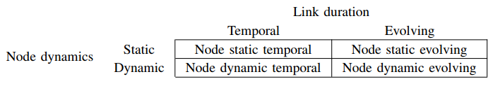
Figure 2: Classifying dynamic networks into four types based on edge duration and node dynamics.
1.2 Representation of Dynamic Networks
Traditional temporal data is generally represented in two ways: discrete and continuous. The former takes equidistant windows along the time axis, aggregating data within the same window into a time step, and finally using discretized time steps to represent continuous temporal data. Continuous representation records the exact time of all data points, preserving all temporal information. Similarly, the representation of dynamic networks is also mainly divided into discrete and continuous forms.
The discrete representation of dynamic networks essentially uses an ordered sequence of static networks to represent dynamic networks. This static network sequence can be viewed as a series of snapshots (Snapshot) of the dynamic network at time steps along the time axis (it can also be represented as a multilayer network or tensor). This representation method is simple, intuitive, and can painlessly utilize GNNs designed for static networks to process these snapshots, thus completing the processing of dynamic network data. However, this representation method inevitably loses temporal information, and the choice of time step length cannot balance computational efficiency and accuracy.
The continuous representation of dynamic networks aims to record the start and end times of all dynamic transformations (or events), thereby retaining all temporal information. It is mainly divided into three forms:
1) Evolving networks can be represented as a collection of tuples, wherein each element records the two endpoints of a dynamic edge, the appearance time, and duration. This representation method is called “event-based representation”;
2) If the duration of edges is too short or not important, it can be omitted based on necessity, and such sequences are referred to as “contact sequences”;
3) When specific time is not important, only relative time matters, a simple ordered edge sequence can represent dynamic networks, which is called “graph stream”.
The choice of which representation method to use is related to the actual data and research focus. While continuous representation retains the temporal information to the greatest extent, it makes the data difficult to process and cannot simply adapt static network representation methods.
Moreover, whether to represent a real dynamic network as discrete or continuous also depends on the dynamic characteristics of the network itself. For temporal networks, continuous representation is more suitable; for evolving networks, discrete representation is more convenient. Readers may consider the reasons behind this.
2. Dynamic Graph Neural Networks (DGNN)
The graph neural networks considered in this article specifically refer to GNNs with domain aggregation operations, which belong to a subfield of network representation learning. Readers interested in the overall research on dynamic networks in the field of graph representation learning can refer to the review published in the Journal of Machine Learning Research in 2019.
As mentioned in the previous subsection, dynamic networks can generally be represented in discrete and continuous forms. According to the different forms of dynamic network data they can handle, the current work on dynamic graph neural networks can be mainly divided into discrete and continuous categories, with a majority focusing on discrete data. The following diagram also includes a classification called pseudo-dynamic (Pseudo-dynamic), which models dynamic processes but does not fit real data, and will not be considered further in the following text. For specific work, please refer to the work of Da Xu et al. in 2019.
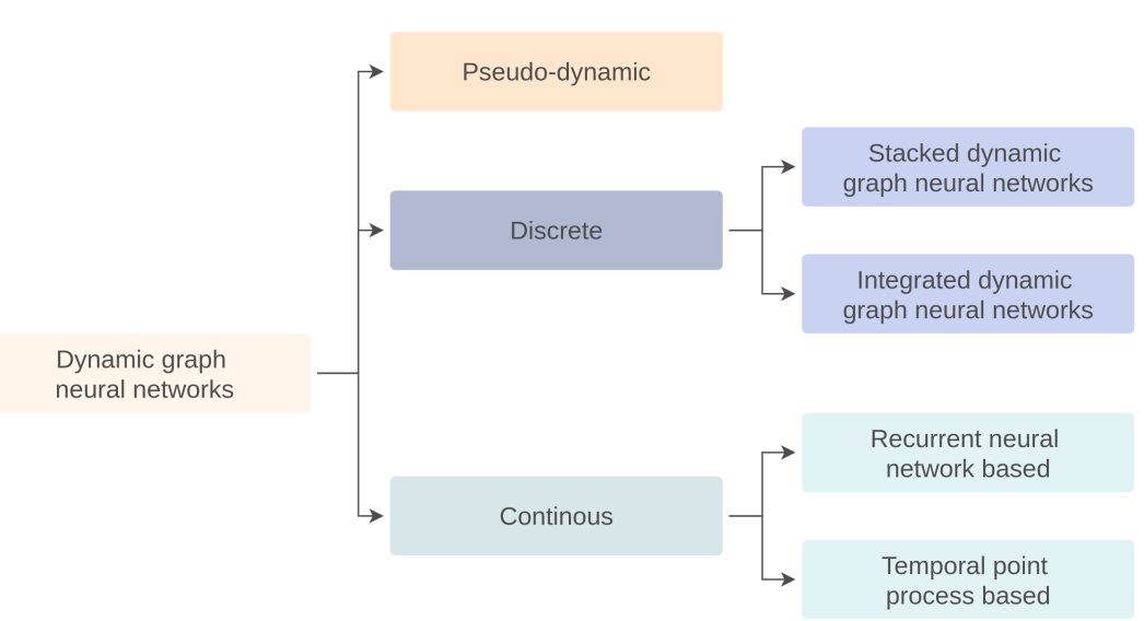
Figure 3: Classification of dynamic graph neural networks.
As the name suggests, discrete DGNN is a framework designed to handle discrete representations of network data. This type of framework is divided into two key modules: 1) For static networks at a single time step, classical GNN models such as GCN and GAT are generally used directly; 2) For capturing discrete temporal information, RNN architectures are typically employed. Self-attention architectures can also be used to capture temporal information.
As shown in the figure above, the discrete DGNN architecture using GNN+RNN is mainly divided into two categories: one is called stacked dynamic GNN (Stacked dynamic gnn), and the other is called integrated dynamic GNN (Integrated dynamic gnn). The main difference between the two lies in how the GNN module and the RNN module are integrated.
2.1.1 Stacked Dynamic Networks
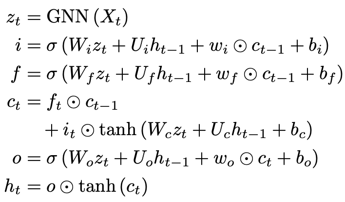
The basic idea of stacked dynamic networks is to use GNN to encode the information of the graph at a single moment, and then use the gating mechanism of RNN (typically LSTM) to complete the transmission and encoding of graph information along the time axis. The overall structure is formed by stacking GNN and RNN sequentially. The simplest form is as follows:
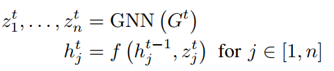
Here, GNN is used to process the static network at time t, combined with the hidden state of RNN to update the node representations. Here, f() represents the RNN structure. Youngjoo et al. introduced the earliest version of this framework in their 2018 work, utilizing GNN and peephole LSTM:
Of course, under the guidance of the above basic idea, stacked dynamic networks can have many variants, including but not limited to using different GNN or RNN models, not sharing RNN parameters between different nodes, and using self-attention mechanisms instead of RNN, etc. Interested readers can refer to the original review for more details.
2.1.2 Integrated Dynamic Networks
The basic idea of integrated dynamic networks is to integrate the GNN module and the RNN module into the same architecture: on the one hand, graph convolution can replace the linear transformation module in RNN, or RNN can control the parameters of GNN at different time steps. Two typical works are:
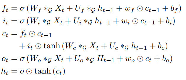
One is a convolutional long short-term memory network (convLSTM) that replaces the linear transformation in LSTM with graph convolution operations, as shown below, where * denotes graph convolution. This variant of LSTM is naturally capable of processing time series composed of graph data.
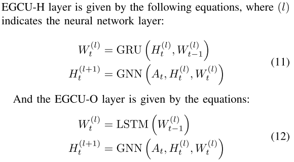
The second work is EvolveGCN proposed in 2019. The starting point of this work is quite simple: it believes that the parameters of GCN processing time series should also evolve (be different) over time. They use RNN to control and update the parameters of GCN at different time steps, as shown in the following diagram.
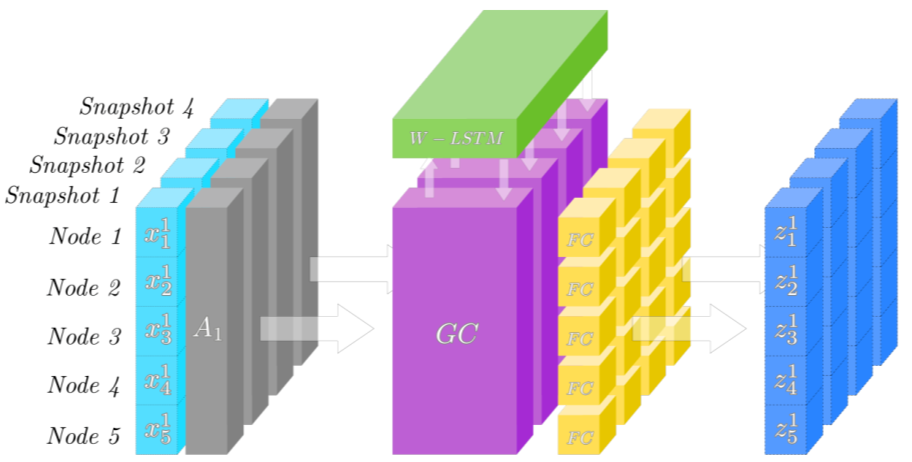
Figure 4: Schematic diagram of the EvolveGCN architecture.
Here, the parameters of GCN can be seen as the hidden state or output of RNN. Based on this idea, they proposed two variants, using the hidden state (EGCU-H) and output (EGCU-O) of RNN to control the parameters of GCN at each step, as shown below:
Additionally, there are some works utilizing Autoencoder, VGAE, and GAN to complete discrete dynamic representations. Interested readers can refer to the original text for more details.
For continuous representations of dynamic networks, current work is also mainly concentrated in two areas: one is RNN-based frameworks, where the representation information of nodes is transmitted and maintained by RNN; the other is frameworks based on temporal point sequences (Temporal point process, TTP), which fit the data by parameterizing TTP using neural networks.
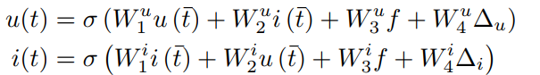
1) RNN-based frameworks: The starting point of this type of work is straightforward; it believes that whenever a change (or event) occurs, the nodes involved in the transformation also need to be updated, so that the node embeddings are continuously updated. Under this framework, there are two main works: one is based on graph streams from JD in 2018, where their framework consists of three parts: (i) interact unit, (ii) update/propagate unit, (iii) merge unit, to complete the update of node embeddings due to an event. The core component is the update/propagate part, which utilizes time-aware LSTM for modeling; the second work is JODIE from Stanford University by Jure in 2019, which considers a bipartite graph between customers u and products i, using two RNNs to control the temporal information of customer and product nodes, respectively. When a new transaction occurs, the corresponding product and user node features are updated immediately:
2) TTP-based frameworks: Temporal point sequences (TTP) are traditional models for modeling asynchronous time series. Continuous dynamic networks are typical asynchronous sequences in a continuous time domain. The work DyRep in 2019 utilizes neural networks to parameterize TTP, allowing it to capture the dynamics of network structure evolution and node dynamics through optimization, achieving richer network representation results by simultaneously modeling these two co-evolving processes. DyRep is also the only framework capable of predicting event occurrence times (others can only predict when events happen). Recent works have also attempted to use NRI and self-attention to better model the TTP process. Additionally, other temporal models have been attempted to model dynamic networks, such as the 2020 work GHN, which used the Hawkes model.
In summary, continuous DGNN can currently only handle specific types of continuous dynamic networks, such as interaction networks and graph stream networks. More general DGNNs capable of solving a wider range of problems are yet to be developed.
3. Decoding and Structural Prediction of Dynamic Network Representations
Finally, the review summarizes how to design decoders and loss functions to utilize the representation results from the above DGNN framework for dynamic link prediction tasks. This section mainly discusses how to perform negative sampling and compute the model’s constraint terms; interested readers can refer to the original text.
Additionally, the authors emphasize that link prediction tasks are extremely imbalanced classification tasks, so care must be taken when selecting performance metrics. The authors also summarize some available performance metrics as follows:
1) AUC: A common metric for classification performance;
2) An improved version of AUC, PRAUC: Yang et al. found that using AUC as a performance metric for link prediction is not very distinguishing due to the imbalanced nature of link prediction. They proposed using Precision and Recall as the x and y coordinates, respectively, to calculate the area under them, PRAUC, as a replacement for the traditional AUC;
3) Precision@K: This metric can overcome the instability caused by AUC’s sensitivity to thresholds, but selecting the value of k is not easy;
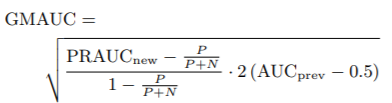
4) GMAUC: Junuthula further improved AUC, suggesting that dynamic link prediction tasks can be decomposed into two sub-tasks: predicting the disappearance/reappearance of edges that have already appeared and predicting edges that have not yet appeared. The first task does not have an imbalance issue and can be measured using AUC; the latter requires PRAUC. By combining both, they proposed a more comprehensive metric GMAUC:
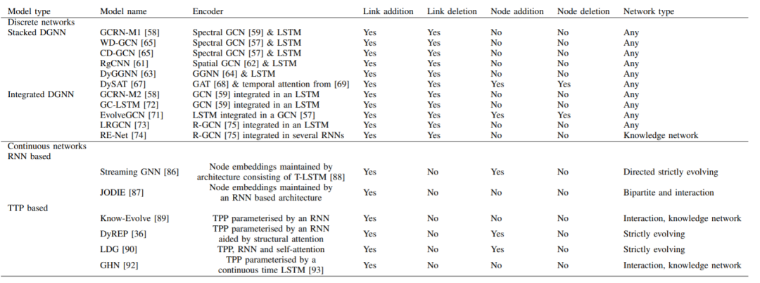
The DGNNs mentioned above, along with the dynamic network tasks and types they can handle, are summarized in the following table:
Table 1: All DGNNs mentioned above and the dynamic network tasks and types they can handle:
Author: Gao Fei
Editor: Zhang Shuang
Latest papers on graph networks from Stanford ICLR 2019: How strong is the representation ability of graph neural networks?
DeepMind again publishes in Nature to solve physical problems, showcasing the powerful capabilities of graph neural networks.
Building bridges between graphs and networks: Where is the next breakthrough in network science?
Beyond Simple Rules – Using Graph Neural Networks for Automatic Modeling of Complex Systems.
Join Intelligent Graph Club and explore complexity together!

Intelligent Graph Club QQ Group | 877391004
Business Cooperation and Submission | [email protected]
Search for the public account: Intelligent Graph Club
Join the “Wall-less Research Institute”
Let the apples fall harder!
👇 Click “Read the original text” to obtain the complete list of paper materials.