Introduction
The concept of deep learning originates from the study of artificial neural networks. A multi-layer perceptron with multiple hidden layers is a type of deep learning structure. Deep learning combines low-level features to form more abstract high-level representations of attribute categories or features, in order to discover distributed feature representations of data. The concept of deep learning was proposed by Hinton et al. in 2006. Based on the Deep Belief Network (DBN), a non-supervised greedy layer-wise training algorithm was proposed, bringing hope to solve the optimization problems related to deep structures. Subsequently, multi-layer autoencoders were introduced as deep structures. Additionally, the convolutional neural network proposed by Lecun et al. is the first true multi-layer structure learning algorithm, which reduces the number of parameters by utilizing spatial relationships to improve training performance. Deep learning is a new field of research in machine learning, motivated by the aim to establish and simulate neural networks that analyze and learn like the human brain, mimicking its mechanisms to interpret data such as images, sounds, and text. Like machine learning methods, deep learning methods can be categorized into supervised and unsupervised learning. The learning models established under different learning frameworks vary significantly. For example, convolutional neural networks (CNNs) are a type of machine learning model under deep supervised learning, while deep belief networks (DBNs) are a type of machine learning model under unsupervised learning.
Deep learning (Deep Learning) has become a hot topic in the field of machine learning in recent years, achieving breakthrough progress in areas such as speech recognition and image recognition. Tencent provides a wide range of internet services, with WeChat having 396 million monthly active users, QQ having 848 million, and Qzone having 644 million monthly active users in the first quarter of 2014. With a vast amount of data and numerous applications, deep learning has extensive potential application scenarios at Tencent.
Deep learning is one of the most noteworthy directions in the field of machine learning in recent years. Since the publication of the paper on Deep Belief Networks [1] by the deep learning pioneer Geoffrey Hinton in Science magazine in 2006, research on neural networks has been revitalized, ushering in a new era of deep neural networks. Both academia and industry are enthusiastic about deep learning, which has gradually achieved breakthrough progress in areas such as speech recognition, image recognition, and natural language processing. Deep learning has achieved a relative accuracy improvement of 20% to 30% in the field of speech recognition, breaking a bottleneck that has lasted nearly a decade. In 2012, deep learning achieved a top-5 accuracy rate of 85% in the ImageNet image classification competition [2], a milestone improvement compared to the 74% accuracy of the previous year, and further improved to 89% in 2013. Major international giants such as Google, Facebook, Microsoft, and IBM, along with domestic internet giants like Baidu and Alibaba, are competing to lay out deep learning.
******************************@*************************************************************************
1. Overview
%%%%%%%%%%%%%%%%%%%%%%%%%%%%%%%%%%%%%%%%%%%%%
2. Background
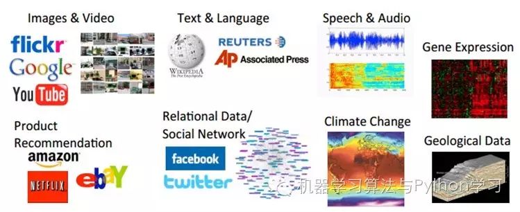
For example, in image recognition, speech recognition, natural language understanding, weather forecasting, gene expression, content recommendation, etc. Currently, the approach we take to solve these problems through machine learning is as follows (using visual perception as an example):
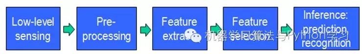
The three middle parts summarize the feature representation. Good feature representation plays a crucial role in the accuracy of the final algorithm, and most of the system’s computational and testing work is spent on this large part. However, this part is generally done manually in practice, relying on manual feature extraction.
However, manually selecting features is a very labor-intensive and heuristic method (requiring expertise), and the ability to select good features largely depends on experience and luck, and its adjustment requires a lot of time. Since manual feature selection is not very effective, can we automatically learn some features? The answer is yes! Deep Learning is designed to do this, as indicated by its alias Unsupervised Feature Learning, which means that no human involvement is required in the feature selection process.
%%%%%%%%%%%%%%%%%%%%%%%%%%%%%%%%%%%%%%%%%%%
3. Visual Mechanism of Human Brain
The Nobel Prize in Physiology or Medicine in 1981 was awarded to David Hubel (a Canadian-born American neurobiologist) and Torsten Wiesel, as well as Roger Sperry. The main contribution of the first two was the “discovery of information processing in the visual system”: the visual cortex is hierarchical:
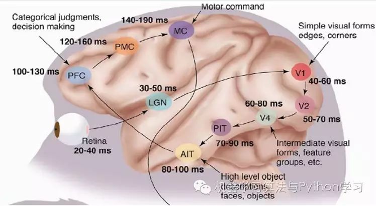
Let’s take a look at what they did. In 1958, David Hubel and Torsten Wiesel at Johns Hopkins University studied the correspondence between the pupil region and cortical neurons in the brain. They made a small hole of 3 mm in the skull of a cat and inserted an electrode into the hole to measure the activity level of the neurons.
Then, they displayed various shapes and brightness levels of objects in front of the kitten. Moreover, they changed the position and angle of the objects while displaying each one. They hoped that through this method, the kitten’s pupil would perceive different types and strengths of stimuli.
The purpose of this experiment was to prove a hypothesis. Different visual neurons located in the occipital cortex correspond to the stimuli received by the pupil in some way. Once the pupil is stimulated by a certain type of stimulus, a specific part of the neurons in the occipital cortex becomes active. After many days of repetitive and tedious experiments, during which several unfortunate kittens were sacrificed, David Hubel and Torsten Wiesel discovered a type of neuron known as “Orientation Selective Cell.” When the pupil detects the edge of an object in front of it, and this edge points in a certain direction, this type of neuron becomes active.
This discovery sparked further thinking about the nervous system. The process of the nervous-central-brain may be a continuously iterative and abstracting process.
There are two keywords here: one is abstraction and the other is iteration. From the original signal, low-level abstraction is gradually iterated to high-level abstraction. Human logical thinking often uses highly abstract concepts.
For example, starting from the intake of the original signal (the pupil receives pixel data), then performing preliminary processing (certain cells in the cortex detect edges and directions), then abstracting (the brain determines that the shape of the object in front is circular), and then further abstracting (the brain further determines that the object is a balloon).
This physiological discovery contributed to the groundbreaking development of artificial intelligence in computer science forty years later.
Sensitive individuals have noticed the keywords: hierarchy. And does the “deep” in Deep Learning indicate how many layers exist, or how deep it is? That’s right. So how does Deep Learning borrow from this process? After all, it is a computer processing problem, and one issue is how to model this process?
Since we need to learn the representation of features, we need to understand features or the hierarchical features in more depth. Therefore, before discussing Deep Learning, it is necessary to elaborate a bit more on features (actually, it seems a bit unfortunate not to include such a good explanation of features here, so I will include it).
%%%%%%%%%%%%%%%%%%%%%%%%%%%%%%%%%%%%%%%%%%%
4. About Characteristics
Features are the raw materials for machine learning systems, and their impact on the final model is unquestionable. If the data is well represented as features, linear models can typically achieve satisfactory accuracy. So what do we need to consider regarding features?
%%%%%%%%%%%%%%%%%%%%%%%%%%%%%%%%%%%%%%%%%%%%
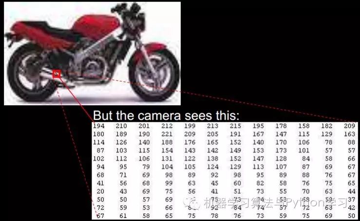
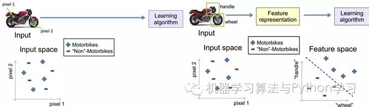
4.1. Granularity of Feature Representation
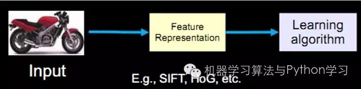
For an image, pixel-level features are of no value at all. For example, in the case of a motorcycle below, pixel-level information cannot provide any information, and it cannot distinguish between a motorcycle and a non-motorcycle. However, if the feature has a structure (or meaning), such as whether it has handlebars or wheels, it becomes very easy to distinguish between a motorcycle and a non-motorcycle, enabling the learning algorithm to function.
%%%%%%%%%%%%%%%%%%%%%%%%%%%%%%%%
4.2. Shallow Feature Representation
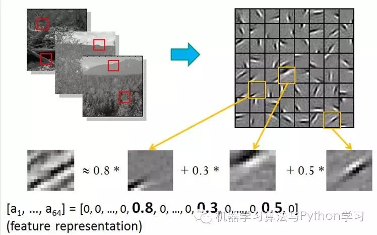
They collected a large number of black-and-white landscape photos and extracted 400 small fragments from these photos, each measuring 16×16 pixels, which can be labeled as S[i], i = 0,.. 399. Next, they randomly extracted another fragment from these black-and-white landscape photos, also measuring 16×16 pixels, and we can label this fragment as T.
The question they posed was how to select a set of fragments, S[k], from these 400 fragments, such that by summing them up, a new fragment is synthesized that is as similar as possible to the randomly selected target fragment T, while keeping the number of S[k] as small as possible. Mathematically, this can be described as:
Sum_k (a[k] * S[k]) –> T, where a[k] is the weight coefficient when summing the fragments S[k].
To solve this problem, Bruno Olshausen and David Field invented an algorithm called sparse coding.
Sparse coding is a repeated iterative process, divided into two steps for each iteration:
1) Select a set of S[k] and then adjust a[k] so that Sum_k (a[k] * S[k]) is as close to T as possible.
2) Fix a[k] and select other more suitable fragments S’[k] from the 400 fragments to replace the original S[k], so that Sum_k (a[k] * S’[k]) is as close to T as possible.
After several iterations, the best combination of S[k] is selected. Surprisingly, the selected S[k] are mostly the edge lines of different objects in the photos, with similar shapes but differing in direction.
The results of Bruno Olshausen and David Field’s algorithm coincided with the physiological findings of David Hubel and Torsten Wiesel!
In other words, complex graphics are often composed of some basic structures. For example, the image below can be linearly represented using 64 orthogonal edges (which can be understood as orthogonal basic structures). For instance, the sample x can be formed by blending three of the edges among the 1-64 edges with weights of 0.8, 0.3, and 0.5, while the other basic edges contribute nothing and are therefore zero.
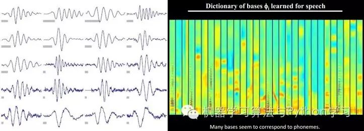
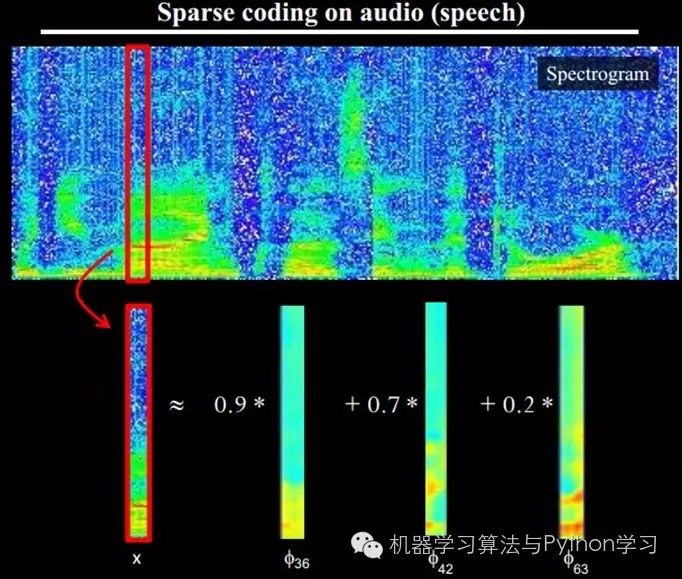
Additionally, researchers have discovered that not only do images exhibit this pattern, but sounds do as well. They found 20 basic sound structures from unlabelled sounds, and the rest of the sounds can be synthesized from these 20 basic structures.
%%%%%%%%%%%%%%%%%%%%%%%%%%%%%%
4.3. Structural Feature Representation
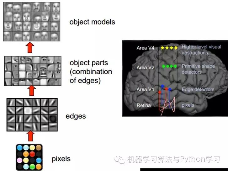
Therefore, V1 looks at the pixel level. V2 looks at V1 at the pixel level; this is a hierarchical progression, with high-level expressions composed of lower-level expressions. More professionally, this is referred to as basis. The basis proposed by V1 is edges, and then the V2 layer is a combination of these bases from the V1 layer, resulting in a higher-level basis obtained from the combination of the previous layer’s bases. The layer above is the result of the combination of the previous layer’s bases… (This is why some experts say Deep Learning is about “basis learning,” which sounds unpleasant, so it is euphemistically called Deep Learning or Unsupervised Feature Learning.)
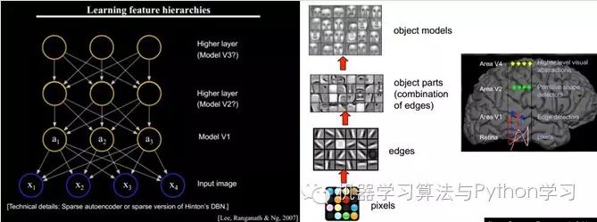
Intuitively, it means finding small patches that make sense and then combining them to obtain the features of the previous layer, recursively learning features upwards.
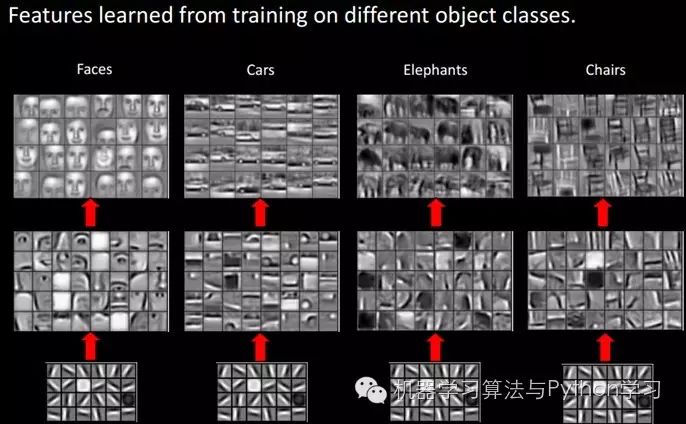
When training on different objects, the obtained edge bases are very similar, but the object parts and models can be completely different (which makes it much easier for us to distinguish between a car or a face):
When a person looks at a document, what the eyes see are words, and from these words, the brain automatically segments them into terms, organizes them according to concepts, learns a priori, obtains topics, and then conducts higher-level learning.
%%%%%%%%%%%%%%%%%%%%%%%%%%%%%%%%%%%%%%%%%%%
4.4. How Many Features Are Needed?
We know that hierarchical feature construction is needed, progressing from shallow to deep, but how many features should each layer have?
Any method with more features provides more reference information, which improves accuracy. However, having too many features means increased computational complexity and a larger exploration space, leading to sparse data for training on each feature, which can cause various issues; thus, more features do not necessarily mean better performance.
Now, at this point, we can finally talk about Deep Learning.
%%%%%%%%%%%%%%%%%%%%%%%%%%%%%%%%%%%%%%%%%%%%
5. Basic Ideas of Deep Learning
Suppose we have a system S, which has n layers (S1,…Sn), with input I and output O, represented as: I =>S1=>S2=>…..=>Sn => O. If the output O equals the input I, it means that no information is lost after the input I passes through this system (Haha, experts say this is impossible. In information theory, there is a saying of “information loss at each layer” (information processing inequality). If processing a information gives b, and then processing b gives c, it can be proven that the mutual information between a and c will not exceed the mutual information between a and b. This indicates that information processing does not increase information, and most processing will lose information. Of course, if what is lost is useless information, that would be great), meaning that at any layer Si, it is another representation of the original information (i.e., input I). Now returning to our topic of Deep Learning, we need to automatically learn features. Suppose we have a batch of input I (like a batch of images or text), and we design a system S (with n layers). By adjusting the parameters in the system, we can ensure that its output is still the input I, allowing us to automatically obtain a series of hierarchical features of the input I, namely S1, …, Sn.
For deep learning, the idea is to stack multiple layers, meaning that the output of one layer serves as the input to the next layer. Through this approach, it is possible to achieve hierarchical expression of the input information.
Additionally, the previous assumption that the output strictly equals the input is too strict; we can slightly relax this condition, for example, we only need to make the difference between input and output as small as possible, which will lead to a different category of Deep Learning methods. The above describes the basic idea of Deep Learning.
%%%%%%%%%%%%%%%%%%%%%%%%%%%%%%%%%%%%%%%%%
6. Shallow Learning vs. Deep Learning
%%%%%%%%%%%%%%%%%%%%%%%%%%%%%%%%
Shallow learning is the first wave of machine learning.
In the late 1980s, the invention of the backpropagation algorithm used for artificial neural networks (also known as the BP algorithm) brought hope to machine learning, sparking a wave of machine learning based on statistical models that continues to this day. It was discovered that using the BP algorithm allows an artificial neural network model to learn statistical patterns from a large number of training samples, thereby predicting unknown events. This statistics-based machine learning method shows superiority in many aspects compared to previous systems based on manual rules. At this time, the artificial neural network, although also referred to as a multi-layer perceptron (MLP), is actually a shallow model containing only one hidden layer of nodes.
In contrast, due to the difficulty of theoretical analysis and the need for a lot of experience and skills in training methods, shallow artificial neural networks were relatively quiet during this period.
%%%%%%%%%%%%%%%%%%%%%%%%%%%%%%%%%%%%%%%%%%%%%%
Deep learning is the second wave of machine learning.
In 2006, Geoffrey Hinton, a professor at the University of Toronto and a pioneer in the field of machine learning, and his student Ruslan Salakhutdinov published a paper in Science that initiated the wave of deep learning in academia and industry. This paper had two main points: 1) Multi-layer artificial neural networks have excellent feature learning capabilities, and the features learned provide a more essential characterization of the data, thus facilitating visualization or classification; 2) The difficulty of training deep neural networks can be effectively overcome through “layer-wise pre-training.” In this paper, layer-wise pre-training is achieved through unsupervised learning.
The essence of deep learning is to construct machine learning models with many hidden layers and massive training data to learn more useful features, ultimately improving classification or prediction accuracy. Therefore, “deep models” are the means, while “feature learning” is the goal. Unlike traditional shallow learning, the differences in deep learning are: 1) It emphasizes the depth of the model structure, typically having 5, 6, or even more than 10 hidden layer nodes; 2) It explicitly highlights the importance of feature learning, meaning that through layer-wise feature transformation, the sample’s feature representation in the original space is transformed into a new feature space, making classification or prediction easier. Compared to methods that construct features using manual rules, utilizing big data to learn features can better capture the rich intrinsic information of the data.
%%%%%%%%%%%%%%%%%%%%%%%%%%%%%%%%%%%%%%%%%%%%%%
7. Deep Learning vs. Neural Networks
Deep learning is a new field of research in machine learning, motivated by the aim to establish and simulate neural networks that analyze and learn like the human brain, mimicking its mechanisms to interpret data such as images, sounds, and text. Deep learning is a type of unsupervised learning.
Deep learning itself can be considered a branch of machine learning, simply understood as the development of neural networks. About two or three decades ago, neural networks were a particularly hot direction in the field of ML, but gradually faded away for several reasons:
1) They are prone to overfitting, parameters are difficult to tune, and many tricks are required;
2) Training speed is relatively slow, and with fewer layers (less than or equal to 3), their performance does not outperform other methods;
Thus, there was a period of about 20 years during which neural networks received little attention; this period was essentially dominated by SVM and boosting algorithms. However, a passionate old gentleman, Hinton, persisted and ultimately (along with others like Bengio and Yann LeCun) proposed a practically feasible deep learning framework.
Deep learning and traditional neural networks have many similarities and differences.
The similarity between the two is that deep learning adopts a hierarchical structure similar to neural networks, consisting of a multi-layer network including input layer, hidden layers (multiple), and output layer, with connections only between adjacent layer nodes, and no connections between nodes in the same layer or across layers. Each layer can be viewed as a logistic regression model; this layered structure closely resembles the structure of the human brain.
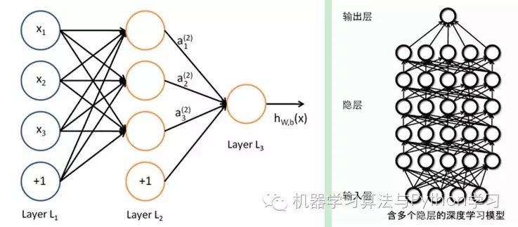
In order to overcome the problems encountered in training neural networks, deep learning adopts a training mechanism that is quite different from neural networks. In traditional neural networks, the backpropagation method is used, which can be simply described as an iterative algorithm to train the entire network, randomly setting initial values, calculating the current output of the network, and then adjusting the parameters of the previous layers based on the difference between the current output and the label, until convergence (the whole process is a gradient descent method). In contrast, deep learning is overall a layer-wise training mechanism. The reason for this is that if the backpropagation mechanism is used for a deep network (more than 7 layers), the residuals propagated back to the front layers become too small, resulting in what is known as gradient diffusion. We will discuss this problem next.
%%%%%%%%%%%%%%%%%%%%%%%%%%%%%%%%%%%%%%%%%%%%%
8. Training Process of Deep Learning
%%%%%%%%%%%%%%%%%%%%%%%%%%%%%%%%
8.1. Why Traditional Neural Network Training Methods Cannot Be Used in Deep Neural Networks
The BP algorithm, as a typical algorithm for training multi-layer networks, is already quite unsatisfactory for networks containing only a few layers. The local minima commonly found in non-convex objective cost functions of deep structures (involving multiple layers of nonlinear processing units) are the main source of training difficulties.
%%%%%%%%%%%%%%
Problems with the BP Algorithm:
(1) Gradients become increasingly sparse: the error correction signals become smaller as they propagate from the top layer downwards;
(2) Convergence to local minima: especially when starting far from the optimal region (random initialization can lead to this situation);
(3) Generally, we can only use labeled data for training: but most data is unlabeled, while the brain can learn from unlabeled data;
%%%%%%%%%%%%%%%%%%%%%%%%%%%%%%%%%%%%%%%%5%%%%%
8.2. The Training Process of Deep Learning
If we train all layers simultaneously, the time complexity will be too high; if we train one layer at a time, the bias will propagate layer by layer. This will face the opposite problem from the supervised learning above, leading to severe underfitting (since the neurons and parameters in deep networks are too many).
In 2006, Hinton proposed an effective method for building multi-layer neural networks on unlabeled data, simply stated, it is divided into two steps: first, train one layer of the network at a time, and second, fine-tune the parameters such that the high-level representation generated from the original representation x and the high-level representation r generated from the high-level representation r are as consistent as possible. The method is as follows:
1) First, progressively build single-layer neurons, training one single-layer network at a time.
2) Once all layers are trained, Hinton uses the wake-sleep algorithm for fine-tuning.
This converts the weights between all layers except the top layer into bidirectional weights, thus keeping the top layer as a single-layer neural network, while the other layers become graphical models. The upward weights are used for “cognition,” and the downward weights are used for “generation.” Then, the Wake-Sleep algorithm adjusts all the weights. This ensures that cognition and generation align, meaning that the generated top-level representation can accurately reconstruct the underlying nodes as closely as possible. For example, if a node in the top layer represents a face, all images of faces should activate this node, and the result generated should represent an approximate facial image.
1) Wake Phase: The cognitive process generates each layer’s abstract representation (node state) through external features and upward weights (cognitive weights), and modifies the downward weights (generative weights) between layers using gradient descent. This means, “If reality differs from my imagination, adjust my weights so that what I imagine aligns with reality.”
2) Sleep Phase: The generative process generates the underlying states through the top-level representations (concepts learned during wakefulness) and downward weights, while modifying the upward weights between layers. This means, “If the scene in my dreams does not correspond to the concept in my mind, adjust my cognitive weights so that this scene appears to be that concept to me.”
%%%%%%%%%%%%%%%%%%%%%%%%%%%%%%%%%%%%%%%%%%%%%%
The specific training process of deep learning is as follows:
1) Use bottom-up unsupervised learning (training from the bottom layer upwards):
The parameters of each layer are trained using unlabeled data (labeled data can also be used). This step can be viewed as an unsupervised training process and is the most significant difference from traditional neural networks (this process can be seen as a feature learning process):
Specifically, first train the first layer using unlabeled data, learning the parameters of the first layer (this layer can be viewed as obtaining a hidden layer of a three-layer neural network that minimizes the difference between output and input). Due to model capacity limitations and sparsity constraints, the resulting model can learn the structure of the data itself, thus obtaining features that have better representation capabilities than the input; after learning the n-1 layer, the output of the n-1 layer is used as the input for the n layer to train the n layer, thus obtaining the parameters for each layer;
2) Top-down supervised learning (training with labeled data, propagating errors from the top down to fine-tune the network):
Based on the parameters obtained in the first step, further fine-tune the parameters of the entire multi-layer model using supervised training; the first step is similar to the random initialization process in neural networks, but since the first step of DL is not random initialization but rather derived from learning the structure of the input data, this initial value is closer to the global optimum, thus achieving better results; hence, the effectiveness of deep learning largely relies on the feature learning process in the first step.
%%%%%%%%%%%%%%%%%%%%%%%%%%%%%%%%%%%%%%%%%%%%
9. Common Models or Methods in Deep Learning
%%%%%%%%%%%%%%%%%%%%%%%%%%%%%%%%%%%%%%%%%%%%%%%%%%%%%
9.1. AutoEncoder
One of the simplest methods in Deep Learning is to utilize the characteristics of artificial neural networks. Artificial neural networks (ANN) themselves are systems with hierarchical structures. If we are given a neural network, we assume its output is the same as its input, and then train and adjust its parameters to obtain the weights in each layer. Naturally, we obtain several different representations of the input I (each layer represents a representation), and these representations are the features. An autoencoder is a neural network that aims to reproduce the input signal as closely as possible. To achieve this reproduction, the autoencoder must capture the most important factors that can represent the input data, just like PCA, finding the main components that can represent the original information.
The specific process is briefly described as follows:
%%%%%%%%%%%%%%%%%%%%%%%%%%%%%%%%%%%%%%%%%%%%%%
1) Given unlabeled data, learn features using unsupervised learning:
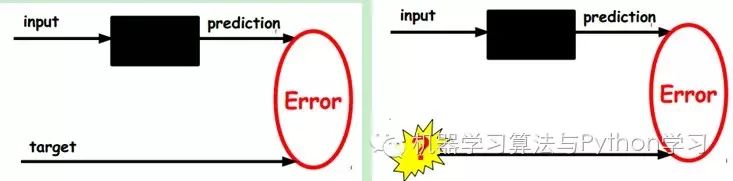
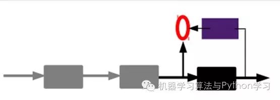
In our previous neural networks, the input samples were labeled, i.e., (input, target), allowing us to adjust the parameters of the previous layers based on the difference between the current output and the target (label) until convergence. But now we only have unlabeled data, i.e., the right-side image. So how do we obtain the error?
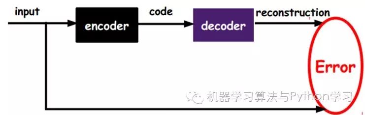
As shown in the image, we input the input into an encoder, which produces a code, which is a representation of the input. How do we know this code represents the input? We add a decoder, and at this point, the decoder outputs information. If the output is very similar to the original input signal (ideally, it is the same), we have reason to believe that this code is reliable. Therefore, we adjust the parameters of the encoder and decoder to minimize the reconstruction error, at which point we obtain the first representation of the input signal, namely the encoding code. Since it is unlabeled data, the source of error is directly obtained by comparing the reconstruction with the original input.
%%%%%%%%%%%%%%%%%%%%%%%%%%%%%%%%
2) Generate features through the encoder, and then train the next layer. This is done layer by layer:
So far, we have obtained the first layer’s code, and minimizing the reconstruction error leads us to believe this code is a good representation of the original input signal, or at least, it is identical (the representations differ but reflect the same thing). The training method for the second layer is no different from the first layer; we take the output code of the first layer as the input signal for the second layer, minimizing the reconstruction error to obtain the parameters for the second layer and the code for the input of the second layer, which is the second representation of the original input information. The same method applies to the other layers (training this layer while keeping the parameters of the previous layers fixed, and their decoders are no longer needed).
%%%%%%%%%%%%%%%%%%%%%%%%%%%%%%
3) Supervised fine-tuning:
After the above methods, we can obtain many layers. As for how many layers are needed (or how deep the depth should be, there is currently no scientific evaluation method), it requires experimentation. Each layer will yield a different representation of the original input. Of course, we believe that the more abstract, the better, just like the human visual system.
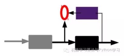
At this point, this AutoEncoder cannot yet be used to classify data, as it has not learned how to connect an input to a class. It has only learned how to reconstruct or reproduce its input. In other words, it has only learned to obtain a feature that can best represent the input signal. To achieve classification, we can add a classifier (such as logistic regression, SVM, etc.) to the top encoding layer of the AutoEncoder, and then train it using standard supervised training methods of multi-layer neural networks (gradient descent method).
In other words, at this point, we need to input the feature code from the last layer into the final classifier, and fine-tune it through labeled samples using supervised learning; this can be done in two ways, one is to adjust only the classifier (the black part):
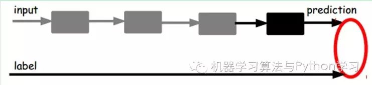
The other way is to fine-tune the entire system through labeled samples (if there is enough data, this is the best. End-to-end learning):

Once the supervised training is complete, this network can be used for classification. The top layer of the neural network can serve as a linear classifier, and we can replace it with a better-performing classifier.
Research has shown that incorporating these automatically learned features into the existing features can significantly improve accuracy, even outperforming the current best classification algorithms!
AutoEncoders have some variants; here are brief introductions to two:
%%%%%%%%%%%%%%%%%%%%%%%%%%%%%%%
Sparse AutoEncoder:
Of course, we can also add some constraints to obtain new Deep Learning methods, such as if we add an L1 regularity constraint to the AutoEncoder (L1 mainly constrains that most nodes in each layer must be zero, with only a few non-zero, hence the name Sparse), we can obtain the Sparse AutoEncoder method.
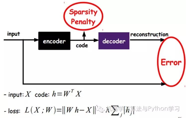
As shown in the image, this actually limits the expressions obtained each time to be as sparse as possible. Sparse representations are often more effective than other representations (it seems the human brain works similarly, where a certain input only stimulates certain neurons, while most other neurons are inhibited).
%%%%%%%%%%%%%%%%%%%%%%%%%%%%%%%%
Denoising AutoEncoders:
Denoising AutoEncoders (DA) build upon the AutoEncoder by adding noise to the training data, forcing the autoencoder to learn to remove this noise to obtain the true input that has not been contaminated by noise. Thus, this compels the encoder to learn a more robust representation of the input signal, which is also the reason for its stronger generalization ability compared to ordinary encoders. DA can be trained using gradient descent algorithms.
%%%%%%%%%%%%%%%%%%%%%%%%%%%%%%%%%%%%%%%%%%%%
 Thank you for your attention and support
Welcome to repost