

This article introduces 7 models for text classification tasks, including traditional bag-of-words models, recurrent neural networks, convolutional neural networks commonly used in computer vision tasks, and RNN + CNN.
This article is based on a previous piece I wrote on sentiment analysis using Twitter data, where I built a simple model: a two-layer feedforward neural network trained with Keras. I used a weighted average of the word embeddings that make up the tweets as the document vector to represent the input tweets.
The embeddings I used were trained from scratch using Gensim based on the corpus. It was a binary classification task, achieving an accuracy of 79%.
The goal of this article is to explore other NLP models trained on the same dataset and evaluate their performance on a given test set.
We will find out if we can achieve an accuracy higher than 79% through different models (from simple models relying on bag-of-words representation to complex models deploying convolutional/recurrent networks)!
First, we will start with simple models and gradually increase the complexity of the models. This work aims to demonstrate that simple models can also be effective.
I will attempt the following:
-
Logistic regression using word-level n-grams
-
Logistic regression using character-level n-grams
-
Logistic regression using both word-level and character-level n-grams
-
Training a recurrent neural network (bidirectional GRU) without pre-trained word embeddings
-
Training a recurrent neural network using GloVe for pre-trained word embeddings
-
Multi-channel convolutional neural network
-
RNN (bidirectional GRU) + CNN model
At the end of the article, sample code for these NLP techniques will be provided. This code can help you start your own NLP project and achieve optimal results (some of these models are very powerful).
We can also provide a comprehensive benchmark that allows us to discern which model is best suited for predicting sentiment in tweets.
In the related GitHub repository, there are different models, their predictions, and the test set. You can try it yourself and get reliable results.
import os
import re

import warnings
warnings.simplefilter("ignore", UserWarning)
from matplotlib import pyplot as plt
%matplotlib inline


import pandas as pd
pd.options.mode.chained_assignment = None
import numpy as np
from string import punctuation

from nltk.tokenize import word_tokenize

from sklearn.model_selection import train_test_split
from sklearn.feature_extraction.text import TfidfVectorizer
from sklearn.linear_model import LogisticRegression
from sklearn.metrics import accuracy_score, auc, roc_auc_score
from sklearn.externals import joblib

import scipy
from scipy.sparse import hstack
0. Data Preprocessing
You can download the dataset from this link (http://thinknook.com/twitter-sentiment-analysis-training-corpus-dataset-2012-09-22/).
Load the data and extract the required variables (sentiment and sentiment text).
The dataset contains 1,578,614 classified tweets, each labeled with 1 (positive sentiment) and 0 (negative sentiment).
The author suggests using 1/10 of the data for testing, while the rest is used for training.
data = pd.read_csv('./data/tweets.csv', encoding='latin1', usecols=['Sentiment', 'SentimentText'])
data.columns = ['sentiment', 'text']
data = data.sample(frac=1, random_state=42)
print(data.shape)
(1578614, 2)
for row in data.head(10).iterrows():
    print(row[1]['sentiment'], row[1]['text'])
1 http://www.popsugar.com/2999655 keep voting for robert pattinson in the popsugar100 as well!!
1 @GamrothTaylor I am starting to worry about you, only I have Navy Seal type sleep hours.
0 sunburned...no sunbaked!    ow.  it hurts to sit.
1 Celebrating my 50th birthday by doing exactly the same as I do every other day - working on our websites.  It's just another day.
1 Leah and Aiden Gosselin are the cutest kids on the face of the Earth
1 @MissHell23 Oh. I didn't even notice.
0 WTF is wrong with me?!!! I'm completely miserable. I need to snap out of this
0 Was having the best time in the gym until I got to the car and had messages waiting for me... back to the down stage!
1 @JENTSYY oh what happened??
0 @catawu Ghod forbid he should feel responsible for anything!
There is a lot of noise in the tweet data. We removed URLs, hashtags, and user mentions from the tweets to clean the data.
def tokenize(tweet):
    tweet = re.sub(r'http\S+', '', tweet)
    tweet = re.sub(r"#(\w+)", '', tweet)
    tweet = re.sub(r"@(\w+)", '', tweet)
    tweet = re.sub(r'[^\\w\s]', '', tweet)
    tweet = tweet.strip().lower()
    tokens = word_tokenize(tweet)
    return tokens
Save the cleaned data to disk.
data['tokens'] = data.text.progress_map(tokenize)
data['cleaned_text'] = data['tokens'].map(lambda tokens: ' '.join(tokens))
data[['sentiment', 'cleaned_text']].to_csv('./data/cleaned_text.csv')

data = pd.read_csv('./data/cleaned_text.csv')
print(data.shape)
(1575026, 2)
data.head()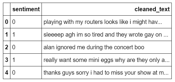
Now that the dataset is cleaned, we can split it into training and testing sets to build the model.
All data in this article is split this way.
x_train, x_test, y_train, y_test = train_test_split(data['cleaned_text'],
                                                    data['sentiment'],
                                                    test_size=0.1,
                                                    random_state=42,
                                                    stratify=data['sentiment'])

print(x_train.shape, x_test.shape, y_train.shape, y_test.shape)
(1417523,) (157503,) (1417523,) (157503,)
Store the test set labels on disk for later use.
pd.DataFrame(y_test).to_csv('./predictions/y_true.csv', index=False)
Next, we can apply machine learning methods.
1. Bag-of-Words Model Based on Word-Level N-grams
So, what is an n-gram?
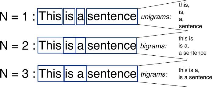
As shown in the figure, an n-gram is all combinations of adjacent words of length n found in the source text.
Our model will use unigrams (n=1) and bigrams (n=2) as features.
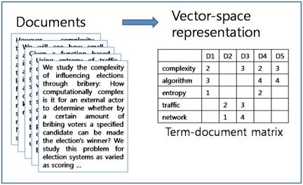
The dataset is represented in a matrix, where each row represents a tweet and each column represents the features extracted from the tweet (after tokenization and cleaning) (unigram model or bigram model). Each cell is the tf-idf score (which can also be simpler values, but tf-idf is more universal and effective). We will call this matrix the document-term matrix.
Upon reflection, the number of unigrams and bigrams after deduplication in a corpus of 1.5 million tweets is still quite large. In fact, for computational power considerations, we can set this number to a fixed value. You can determine this value through cross-validation.
After vectorization, the corpus is as shown in the figure below:
I like pizza a lot
Assuming we use the above features to make predictions for this sentence.
Since we are using the unigram and bigram models, the model extracts the following features:
i, like, pizza, a, lot, i like, like pizza, pizza a, a lot
Thus, the sentence turns into a vector of size N (total number of tokens) containing 0 and the tf-idf scores of these n-grams. So what follows is actually to process this large and sparse vector.
Generally speaking, linear models can handle large and sparse data well. Additionally, linear models train faster compared to other models.
From past experience, logistic regression can work well on sparse tf-idf matrices.
vectorizer_word = TfidfVectorizer(max_features=40000,
                             min_df=5,
                             max_df=0.5,
                             analyzer='word',
                             stop_words='english',
                             ngram_range=(1, 2))

vectorizer_word.fit(x_train, leave=False)

tfidf_matrix_word_train = vectorizer_word.transform(x_train)
tfidf_matrix_word_test = vectorizer_word.transform(x_test)
After generating the tf-idf matrices for the training and testing sets, we can build the first model and test it.
The tf-idf matrix serves as features for logistic regression.
lr_word = LogisticRegression(solver='sag', verbose=2)
lr_word.fit(tfidf_matrix_word_train, y_train)
Once the model is trained, we can apply it to the test data to obtain predictions. Then we will store these values along with the model on disk.
joblib.dump(lr_word, './models/lr_word_ngram.pkl')

y_pred_word = lr_word.predict(tfidf_matrix_word_test)
pd.DataFrame(y_pred_word, columns=['y_pred']).to_csv('./predictions/lr_word_ngram.csv', index=False)
Obtaining the accuracy:
y_pred_word = pd.read_csv('./predictions/lr_word_ngram.csv')
print(accuracy_score(y_test, y_pred_word))
0.782042246814
The first model achieved an accuracy of 78.2%! Not bad. Let’s move on to the second model.
2. Bag-of-Words Model Based on Character-Level N-grams
We never said that n-grams are only for words; they can also be applied to characters.
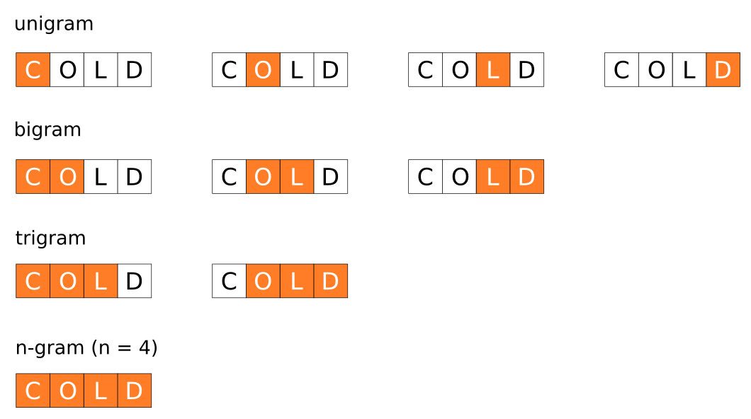
As you can see, we will use the same code for character-level n-grams as shown in the figure, and now we will directly look at 4-grams modeling.
This basically means that a sentence like “I like this movie” will have the following features:
I, l, i, k, e, …, I li, lik, like, …, this, … , is m, s mo, movi, …
Character-level n-grams are effective and can even outperform word-level n-grams in language modeling tasks. Tasks like spam filtering or natural language recognition heavily rely on character-level n-grams.
Unlike the previous models that learned word combinations, this model learns letter combinations, allowing it to handle morphological structures of words.
One advantage of character-based representations is that they can better address spelling errors in words.
Let’s run the same process:
vectorizer_char = TfidfVectorizer(max_features=40000,
                             min_df=5,
                             max_df=0.5,
                             analyzer='char',
                             ngram_range=(1, 4))

vectorizer_char.fit(tqdm_notebook(x_train, leave=False));

tfidf_matrix_char_train = vectorizer_char.transform(x_train)
tfidf_matrix_char_test = vectorizer_char.transform(x_test)

lr_char = LogisticRegression(solver='sag', verbose=2)
lr_char.fit(tfidf_matrix_char_train, y_train)

y_pred_char = lr_char.predict(tfidf_matrix_char_test)
joblib.dump(lr_char, './models/lr_char_ngram.pkl')

pd.DataFrame(y_pred_char, columns=['y_pred']).to_csv('./predictions/lr_char_ngram.csv', index=False)
y_pred_char = pd.read_csv('./predictions/lr_char_ngram.csv')
print(accuracy_score(y_test, y_pred_char))
0.80420055491
80.4% accuracy! The character-level n-gram model performs better than the word-level n-gram.
3. Bag-of-Words Model Based on Both Word-Level and Character-Level N-grams
Compared to the features of word-level n-grams, character-level n-gram features seem to provide better accuracy. So how about combining character-level n-grams with word-level n-grams?
We will concatenate the two tf-idf matrices to create a new, mixed tf-idf matrix. This model helps in learning the morphological structure of words and the morphological structure of words that are likely to be adjacent to this word.
Combine these attributes.
tfidf_matrix_word_char_train =  hstack((tfidf_matrix_word_train, tfidf_matrix_char_train))
tfidf_matrix_word_char_test =  hstack((tfidf_matrix_word_test, tfidf_matrix_char_test))

lr_word_char = LogisticRegression(solver='sag', verbose=2)
lr_word_char.fit(tfidf_matrix_word_char_train, y_train)

y_pred_word_char = lr_word_char.predict(tfidf_matrix_word_char_test)
joblib.dump(lr_word_char, './models/lr_word_char_ngram.pkl')

pd.DataFrame(y_pred_word_char, columns=['y_pred']).to_csv('./predictions/lr_word_char_ngram.csv', index=False)
y_pred_word_char = pd.read_csv('./predictions/lr_word_char_ngram.csv')
print(accuracy_score(y_test, y_pred_word_char))
0.81423845895
Achieved an accuracy of 81.4%. This model added just one overall unit, but the result is better than the previous two.
About bag-of-words models
-
Advantages: Considering its simple nature, bag-of-words models are already quite powerful; they train quickly and are easy to understand.
-
Disadvantages: Even though n-grams carry some context between words, bag-of-words models cannot model long-term dependencies between words in the sequence.
Now we will use deep learning models. The performance of deep learning models surpasses that of bag-of-words models because deep learning models can capture the sequential dependencies of words in sentences. This may be attributed to the emergence of a special neural network structure known as recurrent neural networks.
This article does not cover the theoretical foundations of RNNs, but the content in this link (http://colah.github.io/posts/2015-08-Understanding-LSTMs/) is worth reading. This article originates from Cristopher Olah’s blog, which details a special type of RNN model: Long Short-Term Memory networks (LSTM).
Before we begin, we need to set up an environment dedicated to deep learning to use Keras on TensorFlow. To be honest, I tried running this code on my personal laptop, but considering the size of the dataset and the complexity of the RNN architecture, it was impractical. Another good option is AWS. I generally use the deep learning AMI on EC2 p2.xlarge instances (https://aws.amazon.com/marketplace/pp/B077GCH38C?qid=1527197041958&sr=0-1&ref_=srh_res_product_title). Amazon’s AMI is a pre-configured VM image that has all packages installed (TensorFlow, PyTorch, Keras, etc.). I highly recommend using it!
from keras.preprocessing.text import Tokenizer
from keras.preprocessing.text import text_to_word_sequence
from keras.preprocessing.sequence import pad_sequences

from keras.models import Model
from keras.models import Sequential

from keras.layers import Input, Dense, Embedding, Conv1D, Conv2D, MaxPooling1D, MaxPool2D
from keras.layers import Reshape, Flatten, Dropout, Concatenate
from keras.layers import SpatialDropout1D, concatenate
from keras.layers import GRU, Bidirectional, GlobalAveragePooling1D, GlobalMaxPooling1D

from keras.callbacks import Callback
from keras.optimizers import Adam

from keras.callbacks import ModelCheckpoint, EarlyStopping
from keras.models import load_model
from keras.utils.vis_utils import plot_model
4. Recurrent Neural Network Without Pre-Trained Word Embeddings
RNNs may seem intimidating. Although they are complex and difficult to understand, they are very interesting. RNN models encapsulate a very elegant design to overcome the shortcomings of traditional neural networks when processing sequential data (text, time series, video, DNA sequences, etc.).
RNNs are a series of neural network modules that connect to each other like a chain. Each passes messages backward. I strongly recommend delving into its internal mechanisms from Colah’s blog; the following figure is sourced from there.
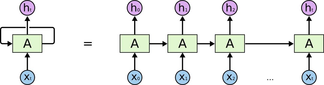
The type of sequence we are dealing with is text data. For meaning, the order of words is crucial. RNNs take this into account, allowing them to capture long-term dependencies.
To use Keras on text data, we first need to preprocess the data. This can be done using Keras’s Tokenizer class. This object uses num_words as a parameter, which is the maximum number of words to keep based on frequency after tokenization.
MAX_NB_WORDS = 80000
tokenizer = Tokenizer(num_words=MAX_NB_WORDS)

tokenizer.fit_on_texts(data['cleaned_text'])
Once the tokenizer is applied to the data, we can convert the text character-level n-grams into numerical sequences using the tokenizer.
These numbers represent the position of each word in the dictionary (think of it as a mapping).
As shown in the example below:
x_train[15]
'breakfast time happy time'
This illustrates how the tokenizer converts it into numerical sequences.
tokenizer.texts_to_sequences([x_train[15]])
[[530, 50, 119, 50]]
Next, apply this tokenizer to the training and testing sequences:
train_sequences = tokenizer.texts_to_sequences(x_train)
test_sequences = tokenizer.texts_to_sequences(x_test)
This maps the tweets to integer lists. However, since the lengths are different, we still cannot stack them in a matrix. Fortunately, Keras allows us to pad the sequences to the maximum length with 0s. We will set this length to 35 (which is the maximum number of tokens in the tweets).
MAX_LENGTH = 35
padded_train_sequences = pad_sequences(train_sequences, maxlen=MAX_LENGTH)
padded_test_sequences = pad_sequences(test_sequences, maxlen=MAX_LENGTH)
padded_train_sequences
array([[    0,     0,     0, ...,  2383,   284,     9],
       [    0,     0,     0, ...,    13,    30,    76],
       [    0,     0,     0, ...,    19,    37, 45231],
       ...,
       [    0,     0,     0, ...,    43,   502,  1653],
       [    0,     0,     0, ...,     5,  1045,   890],
       [    0,     0,     0, ..., 13748, 38750,   154]])
padded_train_sequences.shape
(1417523, 35)
Now we can feed the data into the RNN.
Here are some elements of the architecture I will use:
-
Embedding dimension of 300. This means that each of the 80,000 words we use is mapped to a 300-dimensional dense (floating-point) vector. This mapping will be adjusted during training.
-
Applying a spatial dropout layer on the embedding layer to reduce overfitting: looking at the 35*300 matrix by batches, randomly deleting (setting to 0) the word vectors (rows) in each matrix. This helps keep the model from focusing too much on specific words, which is beneficial for generalization.
-
Bidirectional Gated Recurrent Units (GRU): This is the recurrent network part. It is a faster variant of the LSTM architecture. Think of it as a combination of two recurrent networks, allowing it to scan the text sequence from both directions: left to right and right to left. This allows the network to understand the text by combining the context before and after a given word. The output h_t of each network block in the GRU has a dimension equal to the number of units, which we will set to 100. Since we are using a bidirectional GRU, the final output of each RNN block will be 200-dimensional.
The output of the bidirectional GRU is dimensional (batch size, time steps, and units). This means that if we use a classic batch size of 256, the dimensions will be (256, 35, 200).
-
Global average pooling is applied on each batch, which contains the average value of the output vectors corresponding to each time step (i.e., word).
-
We apply the same operation, but with max pooling instead of average pooling.
-
The outputs of the first two operations are concatenated.
def get_simple_rnn_model():
    embedding_dim = 300
    embedding_matrix = np.random.random((MAX_NB_WORDS, embedding_dim))

    inp = Input(shape=(MAX_LENGTH, ))
    x = Embedding(input_dim=MAX_NB_WORDS, output_dim=embedding_dim, input_length=MAX_LENGTH,
                  weights=[embedding_matrix], trainable=True)(inp)
    x = SpatialDropout1D(0.3)(x)
    x = Bidirectional(GRU(100, return_sequences=True))(x)
    avg_pool = GlobalAveragePooling1D()(x)
    max_pool = GlobalMaxPooling1D()(x)
    conc = concatenate([avg_pool, max_pool])
    outp = Dense(1, activation="sigmoid")(conc)

    model = Model(inputs=inp, outputs=outp)
    model.compile(loss='binary_crossentropy',
                  optimizer='adam',
                  metrics=['accuracy'])
    return model

rnn_simple_model = get_simple_rnn_model()
The different layers of this model are as follows:
plot_model(rnn_simple_model,
           to_file='./images/article_5/rnn_simple_model.png',
           show_shapes=True,
           show_layer_names=True)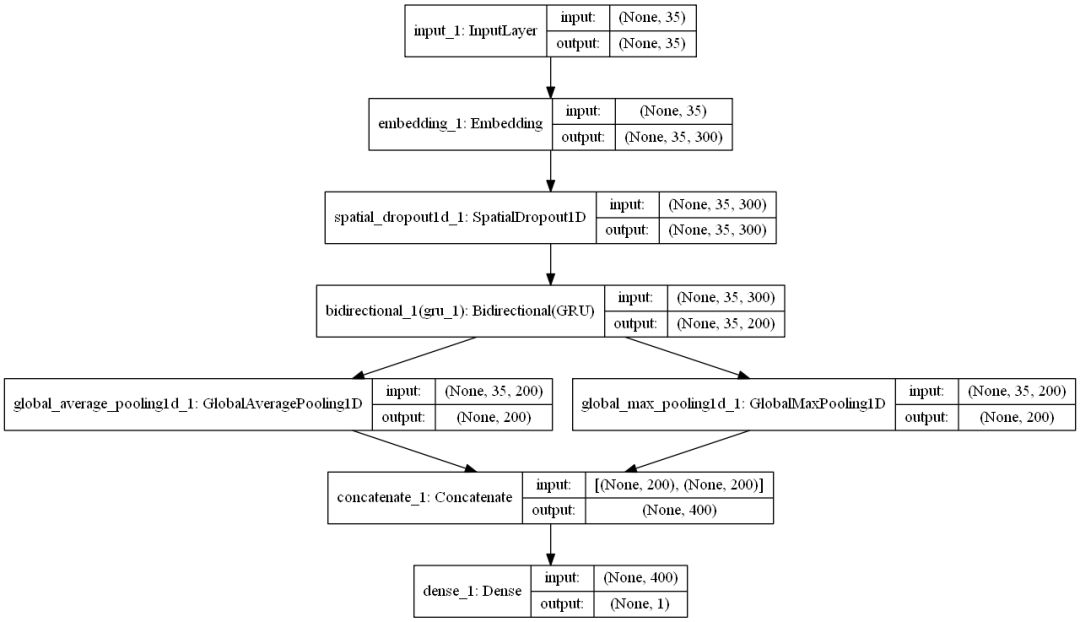
During training, model checkpoints were used. This allows the best model (measured by accuracy) to be automatically stored (on disk) at the end of each epoch.
filepath="./models/rnn_no_embeddings/weights-improvement-{epoch:02d}-{val_acc:.4f}.hdf5"
checkpoint = ModelCheckpoint(filepath, monitor='val_acc', verbose=1, save_best_only=True, mode='max')

batch_size = 256
epochs = 2

history = rnn_simple_model.fit(x=padded_train_sequences,
                    y=y_train,
                    validation_data=(padded_test_sequences, y_test),
                    batch_size=batch_size,
                    callbacks=[checkpoint],
                    epochs=epochs,
                    verbose=1)

best_rnn_simple_model = load_model('./models/rnn_no_embeddings/weights-improvement-01-0.8262.hdf5')

y_pred_rnn_simple = best_rnn_simple_model.predict(padded_test_sequences, verbose=1, batch_size=2048)

y_pred_rnn_simple = pd.DataFrame(y_pred_rnn_simple, columns=['prediction'])
y_pred_rnn_simple['prediction'] = y_pred_rnn_simple['prediction'].map(lambda p: 1 if p >= 0.5 else 0)
y_pred_rnn_simple.to_csv('./predictions/y_pred_rnn_simple.csv', index=False)
y_pred_rnn_simple = pd.read_csv('./predictions/y_pred_rnn_simple.csv')
print(accuracy_score(y_test, y_pred_rnn_simple))
0.826219183127
The accuracy reached 82.6%! This is a very good result! The current model performs better than the previous bag-of-words models because we have considered the sequential nature of the text.
Can we do better?
5. Recurrent Neural Network with GloVe Pre-Trained Word Embeddings
In the last model, the embedding matrix was randomly initialized. What if we initialize it using pre-trained word embeddings? For example: suppose the word “pizza” appears in the corpus. Following the previous architecture, we can obtain a 300-dimensional random floating-point vector for it. This is certainly good. It is easy to implement, and this embedding can be adjusted during training. But you can also use another model trained on a large corpus to generate word embeddings for “pizza” instead of randomly selected vectors. This is a special case of transfer learning.
Using knowledge from external embeddings can improve the accuracy of RNNs because it integrates relevant new information (vocabulary and semantics) for this word, which is trained and refined based on large-scale data corpora.
The pre-trained embedding we will use is GloVe.
The official description is: GloVe is an unsupervised learning algorithm for obtaining word vector representations. The algorithm is trained based on global word-word co-occurrence data in the corpus, and the resulting representations exhibit interesting linear substructures in the word vector space.
The GloVe embeddings used in this article are trained on a very large dataset, including:
-
840 billion tokens;
-
2.2 million words.
Downloading the compressed file takes 2.03GB. Please note that this file cannot be easily loaded on a standard laptop.
GloVe embeddings have 300 dimensions.
The GloVe embeddings come from raw text data, where each line contains a word and 300 floating-point numbers (corresponding to the embeddings). So first, we need to convert this structure into a Python dictionary.
def get_coefs(word, *arr):
    try:
        return word, np.asarray(arr, dtype='float32')
    except:
        return None, None

embeddings_index = dict(get_coefs(*o.strip().split()) for o in tqdm_notebook(open('./embeddings/glove.840B.300d.txt')))

embed_size=300
for k in tqdm_notebook(list(embeddings_index.keys())):
    v = embeddings_index[k]
    try:
        if v.shape != (embed_size, ):
            embeddings_index.pop(k)
    except:
        pass

embeddings_index.pop(None)
Once the embedding index is created, we can extract all vectors, stack them together, and compute their mean and standard deviation.
values = list(embeddings_index.values())
all_embs = np.stack(values)

emb_mean, emb_std = all_embs.mean(), all_embs.std()
Now we generate the embedding matrix. Initialize the matrix according to the normal distribution with mean=emb_mean and std=emb_std. Iterate over the 80,000 words in the corpus. For each word, if it exists in GloVe, we can get the embedding for that word; if not, we skip it.
word_index = tokenizer.word_index
nb_words = MAX_NB_WORDS
embedding_matrix = np.random.normal(emb_mean, emb_std, (nb_words, embed_size))

oov = 0
for word, i in tqdm_notebook(word_index.items()):
    if i >= MAX_NB_WORDS: continue
    embedding_vector = embeddings_index.get(word)
    if embedding_vector is not None:
        embedding_matrix[i] = embedding_vector
    else:
        oov += 1

print(oov)

def get_rnn_model_with_glove_embeddings():
    embedding_dim = 300
    inp = Input(shape=(MAX_LENGTH, ))
    x = Embedding(MAX_NB_WORDS, embedding_dim, weights=[embedding_matrix], input_length=MAX_LENGTH, trainable=True)(inp)
    x = SpatialDropout1D(0.3)(x)
    x = Bidirectional(GRU(100, return_sequences=True))(x)
    avg_pool = GlobalAveragePooling1D()(x)
    max_pool = GlobalMaxPooling1D()(x)
    conc = concatenate([avg_pool, max_pool])
    outp = Dense(1, activation="sigmoid")(conc)

    model = Model(inputs=inp, outputs=outp)
    model.compile(loss='binary_crossentropy',
                  optimizer='adam',
                  metrics=['accuracy'])
    return model

rnn_model_with_embeddings = get_rnn_model_with_glove_embeddings()

filepath="./models/rnn_with_embeddings/weights-improvement-{epoch:02d}-{val_acc:.4f}.hdf5"
checkpoint = ModelCheckpoint(filepath, monitor='val_acc', verbose=1, save_best_only=True, mode='max')

batch_size = 256
epochs = 4

history = rnn_model_with_embeddings.fit(x=padded_train_sequences,
                    y=y_train,
                    validation_data=(padded_test_sequences, y_test),
                    batch_size=batch_size,
                    callbacks=[checkpoint],
                    epochs=epochs,
                    verbose=1)

best_rnn_model_with_glove_embeddings = load_model('./models/rnn_with_embeddings/weights-improvement-03-0.8372.hdf5')

y_pred_rnn_with_glove_embeddings = best_rnn_model_with_glove_embeddings.predict(
    padded_test_sequences, verbose=1, batch_size=2048)

y_pred_rnn_with_glove_embeddings = pd.DataFrame(y_pred_rnn_with_glove_embeddings, columns=['prediction'])
y_pred_rnn_with_glove_embeddings['prediction'] = y_pred_rnn_with_glove_embeddings['prediction'].map(lambda p:
                                                                                                    1 if p >= 0.5 else 0)
y_pred_rnn_with_glove_embeddings.to_csv('./predictions/y_pred_rnn_with_glove_embeddings.csv', index=False)
y_pred_rnn_with_glove_embeddings = pd.read_csv('./predictions/y_pred_rnn_with_glove_embeddings.csv')
print(accuracy_score(y_test, y_pred_rnn_with_glove_embeddings))
0.837203100893
The accuracy reached 83.7%! Transfer learning from external word embeddings worked! The remaining part of this tutorial will use GloVe embeddings in the embedding matrix.
6. Multi-Channel Convolutional Neural Network
This section experiments with a convolutional neural network structure I learned about (http://www.wildml.com/2015/11/understanding-convolutional-neural-networks-for-nlp/). CNNs are commonly used for computer vision tasks. However, recently, I tried applying them to NLP tasks, and the results were promising.
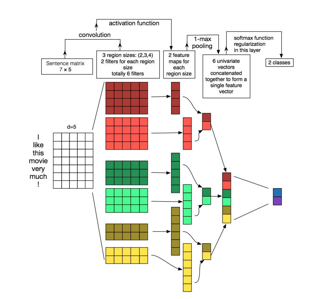
Briefly, let’s see what happens when using convolutional networks on text data. To explain this, I found this very famous image from wildml.com (a great blog).
Consider the example used: I like this movie very much! (7 tokens)
-
The embedding dimension of each word is 5. Hence, the sentence can be represented as a matrix of dimension (7,5). You can think of it as an image (a matrix of numbers or floating points).
-
Six filters, two each of sizes (2, 5), (3, 5), and (4, 5). These filters are applied to the matrix, and their uniqueness lies in the fact that they are not square matrices, but their width equals that of the embedding matrix. Thus, the result of each convolution will be a column vector.
-
Each column vector produced by the convolution is downsampled using max pooling.
-
The results of the max pooling operation are concatenated to form the final vector that will be passed to the softmax function for classification.
What is the principle behind this?
Detecting special patterns will activate the results of each convolution. By varying the sizes of the convolution kernels and connecting their outputs, you can detect patterns of multiple sizes (2, 3, or 5 adjacent words).
Patterns can be expressions like “I hate” or “very good” (word-level n-grams?), thus allowing CNNs to discern them from sentences without considering their positions.
def get_cnn_model():
    embedding_dim = 300

    filter_sizes = [2, 3, 5]
    num_filters = 256
    drop = 0.3

    inputs = Input(shape=(MAX_LENGTH,), dtype='int32')
    embedding = Embedding(input_dim=MAX_NB_WORDS,
                                output_dim=embedding_dim,
                                weights=[embedding_matrix],
                                input_length=MAX_LENGTH,
                                trainable=True)(inputs)

    reshape = Reshape((MAX_LENGTH, embedding_dim, 1))(embedding)
    conv_0 = Conv2D(num_filters,
                    kernel_size=(filter_sizes[0], embedding_dim),
                    padding='valid', kernel_initializer='normal',
                    activation='relu')(reshape)

    conv_1 = Conv2D(num_filters,
                    kernel_size=(filter_sizes[1], embedding_dim),
                    padding='valid', kernel_initializer='normal',
                    activation='relu')(reshape)
    conv_2 = Conv2D(num_filters,
                    kernel_size=(filter_sizes[2], embedding_dim),
                    padding='valid', kernel_initializer='normal',
                    activation='relu')(reshape)

    maxpool_0 = MaxPool2D(pool_size=(MAX_LENGTH - filter_sizes[0] + 1, 1),
                          strides=(1,1), padding='valid')(conv_0)

    maxpool_1 = MaxPool2D(pool_size=(MAX_LENGTH - filter_sizes[1] + 1, 1),
                          strides=(1,1), padding='valid')(conv_1)

    maxpool_2 = MaxPool2D(pool_size=(MAX_LENGTH - filter_sizes[2] + 1, 1),
                          strides=(1,1), padding='valid')(conv_2)
    concatenated_tensor = Concatenate(axis=1)(
        [maxpool_0, maxpool_1, maxpool_2])
    flatten = Flatten()(concatenated_tensor)
    dropout = Dropout(drop)(flatten)
    output = Dense(units=1, activation='sigmoid')(dropout)

    model = Model(inputs=inputs, outputs=output)
    adam = Adam(lr=1e-4, beta_1=0.9, beta_2=0.999, epsilon=1e-08, decay=0.0)

    model.compile(optimizer=adam, loss='binary_crossentropy', metrics=['accuracy'])

    return model

cnn_model_multi_channel = get_cnn_model()

plot_model(cnn_model_multi_channel,
           to_file='./images/article_5/cnn_model_multi_channel.png',
           show_shapes=True,
           show_layer_names=True)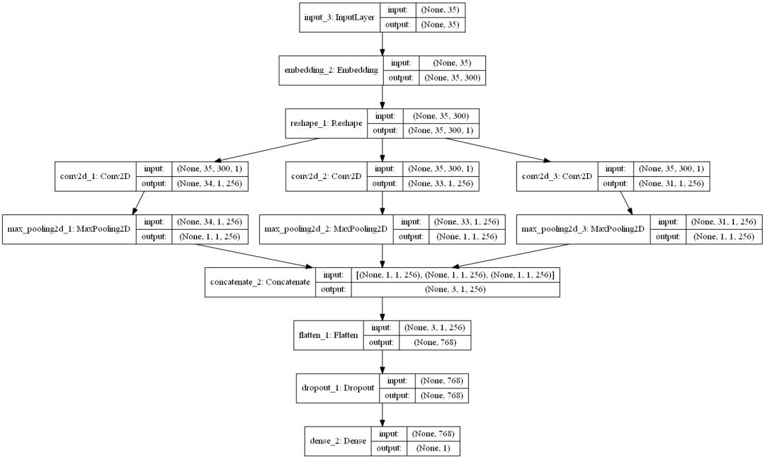
filepath="./models/cnn_multi_channel/weights-improvement-{epoch:02d}-{val_acc:.4f}.hdf5"
checkpoint = ModelCheckpoint(filepath, monitor='val_acc', verbose=1, save_best_only=True, mode='max')

batch_size = 256
epochs = 4

history = cnn_model_multi_channel.fit(x=padded_train_sequences,
                    y=y_train,
                    validation_data=(padded_test_sequences, y_test),
                    batch_size=batch_size,
                    callbacks=[checkpoint],
                    epochs=epochs,
                    verbose=1)

best_cnn_model = load_model('./models/cnn_multi_channel/weights-improvement-04-0.8264.hdf5')

y_pred_cnn_multi_channel = best_cnn_model.predict(padded_test_sequences, verbose=1, batch_size=2048)

y_pred_cnn_multi_channel = pd.DataFrame(y_pred_cnn_multi_channel, columns=['prediction'])
y_pred_cnn_multi_channel['prediction'] = y_pred_cnn_multi_channel['prediction'].map(lambda p: 1 if p >= 0.5 else 0)
y_pred_cnn_multi_channel.to_csv('./predictions/y_pred_cnn_multi_channel.csv', index=False)
y_pred_cnn_multi_channel = pd.read_csv('./predictions/y_pred_cnn_multi_channel.csv')
print(accuracy_score(y_test, y_pred_cnn_multi_channel))
0.826409655689
The accuracy is 82.6%, not as high as the RNN, but still better than the BOW model. Perhaps tuning hyperparameters (number and size of filters) will bring some improvements?
7. RNN + CNN
RNNs are powerful. However, it has been found that stacking convolutional layers on top of recurrent layers can make the network even stronger.
The principle behind this is that RNNs allow embedding sequences and the relevant information of previous words, while CNNs can use these embeddings to extract local features. These two layers working together can be considered a strong combination.
For more information, please refer to: http://konukoii.com/blog/2018/02/19/twitter-sentiment-analysis-using-combined-lstm-cnn-models/
def get_rnn_cnn_model():
    embedding_dim = 300
    inp = Input(shape=(MAX_LENGTH, ))
    x = Embedding(MAX_NB_WORDS, embedding_dim, weights=[embedding_matrix], input_length=MAX_LENGTH, trainable=True)(inp)
    x = SpatialDropout1D(0.3)(x)
    x = Bidirectional(GRU(100, return_sequences=True))(x)
    x = Conv1D(64, kernel_size = 2, padding = "valid", kernel_initializer = "he_uniform")(x)
    avg_pool = GlobalAveragePooling1D()(x)
    max_pool = GlobalMaxPooling1D()(x)
    conc = concatenate([avg_pool, max_pool])
    outp = Dense(1, activation="sigmoid")(conc)

    model = Model(inputs=inp, outputs=outp)
    model.compile(loss='binary_crossentropy',
                  optimizer='adam',
                  metrics=['accuracy'])
    return model

rnn_cnn_model = get_rnn_cnn_model()

plot_model(rnn_cnn_model, to_file='./images/article_5/rnn_cnn_model.png', show_shapes=True, show_layer_names=True)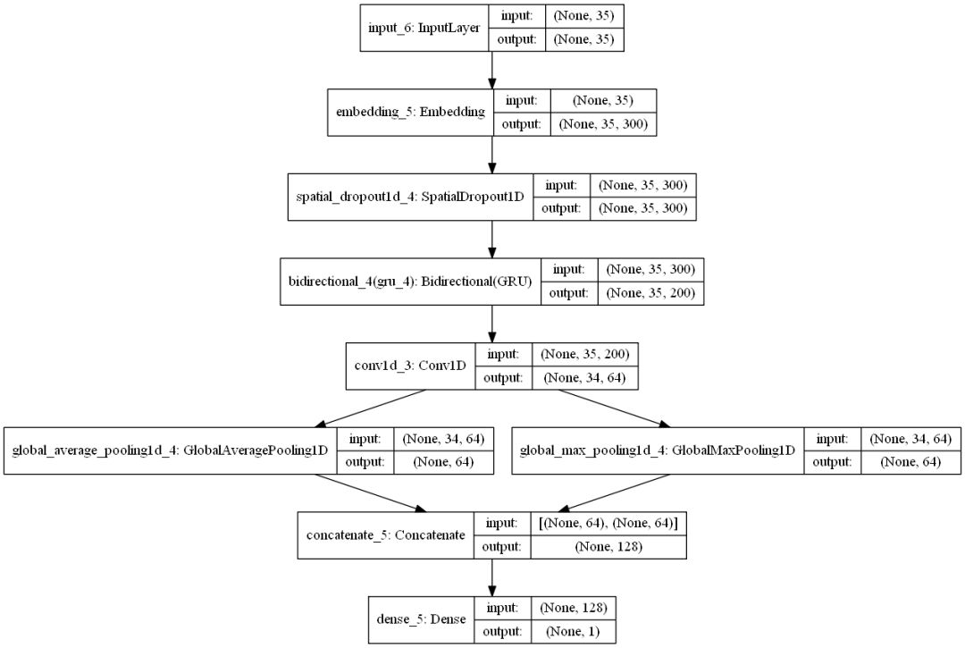
filepath="./models/rnn_cnn/weights-improvement-{epoch:02d}-{val_acc:.4f}.hdf5"
checkpoint = ModelCheckpoint(filepath, monitor='val_acc', verbose=1, save_best_only=True, mode='max')

batch_size = 256
epochs = 4

history = rnn_cnn_model.fit(x=padded_train_sequences,
                    y=y_train,
                    validation_data=(padded_test_sequences, y_test),
                    batch_size=batch_size,
                    callbacks=[checkpoint],
                    epochs=epochs,
                    verbose=1)

best_rnn_cnn_model = load_model('./models/rnn_cnn/weights-improvement-03-0.8379.hdf5')

y_pred_rnn_cnn = best_rnn_cnn_model.predict(padded_test_sequences, verbose=1, batch_size=2048)

y_pred_rnn_cnn = pd.DataFrame(y_pred_rnn_cnn, columns=['prediction'])
y_pred_rnn_cnn['prediction'] = y_pred_rnn_cnn['prediction'].map(lambda p: 1 if p >= 0.5 else 0)
y_pred_rnn_cnn.to_csv('./predictions/y_pred_rnn_cnn.csv', index=False)
y_pred_rnn_cnn = pd.read_csv('./predictions/y_pred_rnn_cnn.csv')
print(accuracy_score(y_test, y_pred_rnn_cnn))
0.837882453033
This yields an accuracy of 83.8%, which is the best result so far.
8. Summary
After running 7 different models, we compared:
import seaborn as sns
from sklearn.metrics import roc_auc_score
sns.set_style("whitegrid")
sns.set_palette("pastel")

predictions_files = os.listdir('./predictions/')

predictions_dfs = []
for f in predictions_files:
    aux = pd.read_csv('./predictions/{0}'.format(f))
    aux.columns = [f.strip('.csv')]
    predictions_dfs.append(aux)

predictions = pd.concat(predictions_dfs, axis=1)

scores = {}

for column in tqdm_notebook(predictions.columns, leave=False):
    if column != 'y_true':
        s = accuracy_score(predictions['y_true'].values, predictions[column].values)
        scores[column] = s

scores = pd.DataFrame([scores], index=['accuracy'])

mapping_name = dict(zip(list(scores.columns),
                        ['Char ngram + LR', '(Word + Char ngram) + LR',
                           'Word ngram + LR', 'CNN (multi channel)',
                           'RNN + CNN', 'RNN no embd.', 'RNN + GloVe embds.']))

scores = scores.rename(columns=mapping_name)
scores = scores[['Word ngram + LR', 'Char ngram + LR', '(Word + Char ngram) + LR',
                'RNN no embd.', 'RNN + GloVe embds.', 'CNN (multi channel)',
                'RNN + CNN']]

scores = scores.T

ax = scores['accuracy'].plot(kind='bar',
                             figsize=(16, 5),
                             ylim=(scores.accuracy.min()*0.97, scores.accuracy.max() * 1.01),
                             color='red',
                             alpha=0.75,
                             rot=45,
                             fontsize=13)
ax.set_title('Comparative accuracy of the different models')

for i in ax.patches:
    ax.annotate(str(round(i.get_height(), 3)),
                (i.get_x() + 0.1, i.get_height() * 1.002), color='dimgrey', fontsize=14)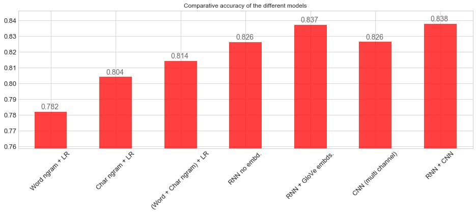
We can quickly see the correlations between the predicted values of these models.
fig = plt.figure(figsize=(10, 5))
sns.heatmap(predictions.drop('y_true', axis=1).corr(method='kendall'), cmap="Blues", annot=True);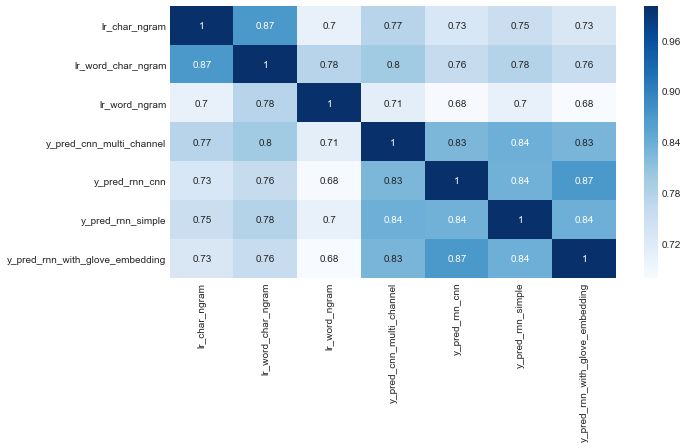
Conclusion
Here are a few findings that I think are worth sharing:
-
Using character-level n-gram bag-of-words models is very effective. Don’t underestimate bag-of-words models; they are low-cost and easy to interpret.
-
RNNs are powerful. But you can also stack external pre-trained embeddings like GloVe on RNN models. Other common embeddings like word2vec and FastText can also be used.
-
CNNs can also be applied to text. The main advantage of CNNs is their fast training speed. Additionally, their ability to extract local features from text is also interesting for NLP tasks.
-
RNNs and CNNs can be stacked together, allowing both structures to be utilized simultaneously.
This article is lengthy, and I hope it can help everyone.
Repository address sharing:

Reply "code" in the backend of the Machine Learning Algorithm and Natural Language Processing public account,
You can get 195 NAACL + 295 ACL2019 papers with open-source code. The open-source address is as follows: https://github.com/yizhen20133868/NLP-Conferences-Code

Important! The Pytorch group for Natural Language Processing has officially been established!
There are a lot of resources in the group, welcome everyone to join the group to learn!
Note: Please modify your remarks to [School/Company + Name + Direction] when adding.
For example - HIT + Zhang San + Dialogue System.
Account holders, please consciously avoid. Thank you!


Recommended reading:
Longformer: A Pre-trained Model for Long Documents Beyond RoBERTa

An Intuitive Understanding of KL Divergence

Top 100 Must-Read Papers on Machine Learning: High Citation, Full Classification, Wide Coverage | GitHub 21.4k Stars