Click the "Xiaobai Learns Vision" above, select "Add to Favorites" or "Pin"
Heavyweight content delivered first time
Introduction This article explains in detail how the minimax game and total loss function in GAN optimization functions are derived. It will introduce the meaning and reasoning of the optimization function in the original GAN, as well as its difference from the model’s total loss function, which is crucial for understanding Generative Adversarial Networks.
Generative Adversarial Networks (GANs) have become very popular in the field of artificial intelligence in recent years, especially in computer vision. With the introduction of the paper “Generative Adversarial Nets” [1], this powerful generative strategy emerged, leading to many research projects that have developed into new applications, such as the latest DALL-E 2[2] or GLIDE[3] (both applications are developed using diffusion models, which are the latest paradigm of generative models. However, GANs remain widely used today).
Introduction to GANs
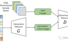
Generative Adversarial Networks (GANs) are a deep learning framework designed as generative models, aiming to generate new complex data (outputs).
To train a GAN, only a set of data to mimic (images, audio, or even tabular data…) is needed. The network will figure out how to create new data that looks like the examples from the provided dataset. In other words, we give the model some example data as input to “get inspired” and let it generate new outputs freely.
Since we only input X information into the network without adding any labels (or expected outputs), this training process is unsupervised learning.
The GAN architecture consists of two competing networks (hence the name “adversarial networks”). These two networks are usually referred to as the Generator (G) and the Discriminator (D). The task of the Generator is to learn the function to generate data starting from random noise, while the Discriminator must decide whether the generated data is “real” (where “real” refers to whether the data belongs to the example dataset). These two networks are trained and learn simultaneously.
There are many different variants of GANs, so training has many different variations. However, if we follow the original paper [1], the training loop of the original GAN is as follows:
For each training iteration, the following operations are performed:
-
Generate m examples (images, audio…) from the represented sample distribution (i.e., random noise z): G(z)
-
Take m samples from the training dataset: x
-
Mix all examples (generated and training dataset) and provide them to the discriminator D. The output of D will be between 0 and 1, indicating that the example is fake, with 1 meaning the example is real.
-
Obtain the discriminator loss function and adjust parameters.
-
Generate new m examples G'(z)
-
Send G'(z) to the discriminator. Obtain the Generator Loss function and adjust parameters.
Note: Generally, we measure the generator loss and adjust its parameters along with the discriminator’s at step 4, allowing us to skip steps 5 and 6, saving time and computational resources.
Optimization Function (Minimax Game) and Loss Function
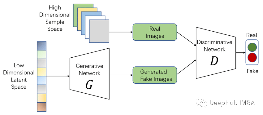
The optimization function of the model in the original GAN paper is as follows:
The above formula is the Optimization function, which is the expression that both networks (Generator and Discriminator) need to optimize. In this case, G wants to minimize it while D wants to maximize it. However, this is not the total loss function of the model.
To understand this minimax game, we need to consider how to measure the model’s performance so that we can optimize it through backpropagation. Since the GAN architecture consists of two simultaneously trained networks, we must calculate two metrics: generator loss and discriminator loss.
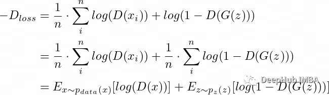
1. Discriminator Loss Function
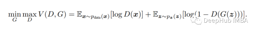
According to the training loop described in the original paper [1], the discriminator receives a batch of m examples from the dataset and another m examples from the generator, outputting a number ∈ [0,1], which indicates the probability that the input data belongs to the dataset distribution (i.e., the probability that the data is “real”).
By knowing which samples are real (samples x from the dataset are real) and which are generated (outputs G(z) from the generator), labels can be assigned: y = 0 (generated), y = 1 (real).
Thus, the discriminator can be trained as a common binary classifier using the binary cross-entropy loss function:

Since this is a binary classifier, we can simplify the following:
– When the input is real data, y = 1 → ∑= log(D(k))
– When the input is data generated by the generator, y = 0 → ∑= log(1-D(k))
The expression can be rewritten in a simpler form:

2. Optimization Function
The discriminator wants to minimize its loss; it aims to minimize the above formula. However, if we modify the formula to remove the “negative sign,” we need to maximize it:

Finally, our operation becomes:
Then we rewrite this formula:

Next, let’s look at the generator’s case: the generator’s goal is to fool the discriminator. The generator must find the minimum value of V(G,D).

Summarizing the two expressions (discriminator and generator optimization functions) gives us the final one:

We have obtained the optimization function. However, this is not the total loss function; it only tells us the overall performance of the model (as the discriminator judges real or fake). If we need to calculate the total loss, we must also add the generator-related part.
3. Generator Loss Function
The generator only participates in the second term of the expression E(log(1-D(G(z)))), while the first term remains unchanged. Therefore, the generator loss function tries to minimize:

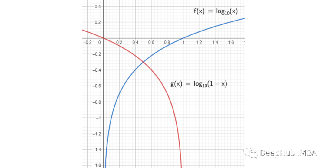
In the original paper, it was mentioned that, “Early in learning, when G is poor, D can reject samples with high confidence because they are clearly different from the training data.” This means that in the early stages of training, the discriminator can easily distinguish between real images and generated images because the generator has not yet learned. In this case, log(1 − D(G(z))) saturates as D(G(z)) ∼ 0.
To avoid this situation, researchers suggested: “We can train G to maximize log D(G(z)) instead of training G to minimize log(1 – D(G(z))).”
This means that instead of training the generator to minimize the probability that the image is fake, we maximize the probability that the image is real. Since essentially these two optimization methods are the same, we can see this in the graph:
The generator loss function used in the paper is:

In practical use, the generator loss function is typically written in the negative form of the above formula, aiming not to maximize the function but to minimize it. This makes it easier to use libraries like TensorFlow to adjust parameters.
Total Loss Function
Above, we have provided the loss formulas for both the generator and the discriminator and given the model’s optimization function. But how do we measure the overall performance of the model?
Simply looking at the optimization function is not a good metric since the optimization function is a modification of the discriminator’s loss function, so it does not reflect the performance of the generator (even though the generator’s loss function originates from it, we only consider the discriminator’s performance in that function). However, if we consider both functions together to evaluate performance, we need to account for the differences between these two functions and make corrections:
a. The two separate loss functions must aim for minimization or maximization. Otherwise, the error reflected in the addition will be higher or lower than it should be. For example, let’s take the optimization function, which aims to be maximized by D:

And the first generator loss function, which aims to minimize G:

When D performs poorly (low error) while G performs well (also low error), the overall performance will yield a low error, which from the metrics means both networks (G and D) are doing well, but in reality, we know one is not.
If one loss aims for minimization while the other aims for maximization, resulting in a high error rate, we also do not know if it is good or bad because the directions of both objectives are different. Moreover, if a loss function aimed at maximization is referred to as “error,” it might sound a bit odd since the “higher” the error, the better the performance. Although we can also use logarithms to convert it, such as log(1+Error).
b. For constructing a total loss function, the individual losses must be within the same value range. Let’s continue to look at the following losses:

And

For the first issue, we have transformed both functions to meet the conditions for minimization. However, the loss of D ranges from [0, +∞], while the output values of G’s loss are in the range (-∞, 0). Adding these two functions effectively removes the influence of the generator’s loss from the discriminator’s loss (i.e., E(log(D(xi))), where E represents the expected value), which is actually incorrect.
What if we use the negative form of the D and modified G losses?

Isn’t this the total loss function of GANs mentioned in the paper? Let’s check if it meets our requirements.
✅ We know the purpose of the D loss is minimization, and the negative form of the modified G loss is also minimization.
✅ The output values of the D loss are in the range [0, +∞), and the negative G loss will also map values to the same range.
Not only are they the same in direction, but also in the value range.
Conclusion
-
The optimization function of GANs (also called the minimax game) and the total loss function are different concepts: minimax optimization ≠ total loss.
-
The origin of the optimization function comes from binary cross-entropy (which in turn is the discriminator loss), and from this, the generator loss function is derived.
-
In practical applications, the generator loss function is modified and logarithmic operations are performed. This modification also helps in calculating the total loss function of the model.
-
Total loss = D loss + G loss. Additionally, to calculate the total loss, modifications were made to ensure that both the direction and value ranges are the same.
Download 1: OpenCV-Contrib Extension Module Chinese Tutorial

Reply "Extension Module Chinese Tutorial" in the background of "Xiaobai Learns Vision" public account to download the first Chinese version of OpenCV extension module tutorial online, covering over twenty chapters including extension module installation, SFM algorithms, stereo vision, object tracking, biological vision, super-resolution processing, etc.

Download 2: Python Vision Practical Project 52 Lectures

Reply "Python Vision Practical Project" in the background of "Xiaobai Learns Vision" public account to download 31 vision practical projects including image segmentation, mask detection, lane line detection, vehicle counting, eyeliner addition, license plate recognition, character recognition, emotion detection, text content extraction, face recognition, etc., to help quickly learn computer vision.

Download 3: OpenCV Practical Project 20 Lectures

Reply "OpenCV Practical Project 20 Lectures" in the background of "Xiaobai Learns Vision" public account to download 20 practical projects based on OpenCV, achieving advanced learning of OpenCV.

Discussion Group

Welcome to join the reader group of the public account to communicate with peers. Currently, there are WeChat groups for SLAM, 3D vision, sensors, autonomous driving, computational photography, detection, segmentation, recognition, medical imaging, GAN, algorithm competitions, etc. (will gradually be subdivided in the future). Please scan the WeChat number below to join the group, remark: "Nickname + School/Company + Research Direction", for example: "Zhang San + Shanghai Jiao Tong University + Vision SLAM". Please follow the format for remarks, otherwise, it will not be approved. After successful addition, you will be invited to the relevant WeChat group based on your research direction. Please do not send advertisements in the group, otherwise, you will be removed from the group. Thank you for your understanding~