

Source: Machine Heart
Author: Jiang Siyuan
The length of this article is 8300 words, recommended reading time is 8 minutes
This article will start from the original paper, using Goodfellow’s speech at NIPS 2016 and Li Hongyi’s explanation from National Taiwan University, to complete the derivation, proof, and implementation of the original GAN.
This article is the second GitHub implementation project of Machine Heart, the previous GitHub implementation project was to build a convolutional neural network from scratch.
This article is mainly divided into four parts:
-
The first part describes the intuitive concept of GAN.
-
The second part describes the formal expression of the concept and optimization.
-
The third part will provide a detailed theoretical derivation and analysis of GAN.
-
Finally, we will implement the theoretical analysis mentioned above.
GitHub project address:
https://github.com/jiqizhixin/ML-Tutorial-Experiment
Basic Concept of Generative Adversarial Networks
To understand generative adversarial models (GAN), we must first understand that generative adversarial models can be divided into two modules: one is the discriminator model, and the other is the generator model. In simple terms: two players compete to see whether A’s attack is stronger or B’s defense is better. For example, we have some real data, as well as some randomly generated fake data. A desperately tries to mimic the real data with the fake data he randomly picked up and mixes it in with the real data. B, on the other hand, tries hard to distinguish between the real data and the fake data.
Here, A is a generator model, similar to a counterfeiter, constantly learning how to deceive B. Meanwhile, B is a discriminator model, akin to an inspector, tirelessly learning how to identify A’s counterfeiting techniques.
As a result, as B’s identification skills improve, A’s counterfeiting skills also become more refined, and a top-notch counterfeiter is what we need. Although the underlying idea of GAN is quite intuitive and simple, we need to further understand the proof and derivation behind this theory.
In summary, GAN proposed by Goodfellow et al. is a new framework for estimating generative models through adversarial processes. In this framework, we need to train two models simultaneously: one generative model G that captures the data distribution and one discriminative model D that estimates the probability that the data comes from real samples. The training process of the generator G maximizes the probability of the discriminator making a mistake, i.e., the discriminator mistakenly believes that the data is real samples rather than fake samples generated by the generator. Therefore, this framework corresponds to a minimax game between two participants. Among all possible functions G and D, we can find a unique equilibrium solution, where G can generate a distribution identical to the training samples, and the probability judged by D is 1/2 everywhere. This process of derivation and proof will be explained in detail later.
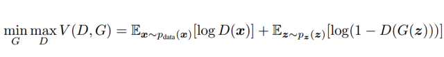
When both models are multilayer perceptrons, the adversarial modeling framework can be applied most directly. To learn the distribution P_g of the generator given data x, we first define a prior input noise variable P_z(z), and then map it to the data space according to G(z;θ_g), where G is a differentiable function represented by a multilayer perceptron. We also need to define a second multilayer perceptron D(s;θ_d), whose output is a single scalar. D(x) represents the probability that x comes from real data rather than P_g. We train D to maximize the probability of correctly assigning real samples and generated samples, so we can simultaneously train G by minimizing log(1-D(G(z))). In other words, the discriminator D and generator engage in a minimax game over the value function V(G,D):
In the latter part, we will conduct a theoretical analysis of adversarial networks. This theoretical analysis essentially indicates that if the model complexities of G and D are sufficient (i.e., under non-parametric constraints), then the adversarial network can generate data distributions. Furthermore, Goodfellow et al. briefly introduced the basic concepts using the following case in their paper.
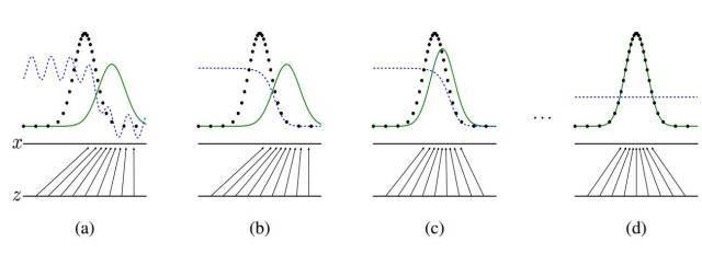
As shown in the figure above, the generative adversarial network trains and updates the discriminative distribution (i.e., D, the blue dashed line). After updating the discriminator, it can distinguish the real distribution of data (the line composed of black dots) from the generative distribution P_g(G) (the green solid line). The horizontal line at the bottom represents the sampling domain Z, where the equidistant lines indicate that samples in Z are uniformly distributed. The upper horizontal line represents a part of the real data X. The upward arrow indicates how the mapping x=G(z) applies an uneven distribution P_g to the noise samples (uniformly sampled). (a) Consider the adversarial training near the convergence point: P_g and P_data are already very similar, and D is a locally accurate classifier. (b) During the internal loop of the algorithm, D is trained to distinguish real samples from data, and this loop will ultimately converge to D(x)=p_data(x)/(p_data(x)+p_g(x)). (c) Then, fix the discriminator and train the generator. After updating G, the gradient of D will guide G(z) towards the direction more likely to be classified as real data by D. (d) After several trainings, if G and D have sufficient complexity, they will reach an equilibrium point. At this point, p_g=p_data, meaning that the probability density function of the generator is equal to that of the real data, i.e., the generated data is the same as the real data. At the equilibrium point, neither D nor G can further improve, and the discriminator cannot determine whether the data comes from real samples or fake data, i.e., D(x)=1/2.
The above briefly introduces the basic concept of generative adversarial networks. The next section will formalize these concepts and describe the general process of optimization.
Formalization of Concepts and Processes
Theoretically Perfect Generator
The goal of the algorithm is to make the generator produce samples that are almost indistinguishable from real data, that is, a top-notch counterfeiter A, which is the generative model we want. Mathematically, this means generating random variables to a certain probability distribution, or saying that the probability density functions are equal: P_G(x)=P_data(x). This is precisely the strategy to prove the efficiency of the generator mathematically: to define an optimization problem where the optimal generator G satisfies P_G(x)=P_data(x). If we know that the solved G will ultimately satisfy this relationship, we can reasonably expect the neural network to obtain the optimal G through typical SGD training.
Optimization Problems
As we initially understood in the case of police and counterfeiters, defining the optimization problem can consist of the following two parts. First, we need to define a discriminator D to determine whether the sample is drawn from P_data(x) distribution, thus:
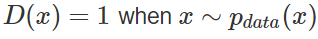
Where E denotes expectation. This term is constructed based on the log loss function for the “positive class” (i.e., distinguishing that x belongs to real data). Maximizing this term means that the discriminator D can accurately predict D(x)=1 when x follows the probability density of data, that is:

Another term is the generator G that attempts to deceive the discriminator. This term is constructed based on the log loss function for the “negative class”, that is:

Since log(x)<1 is negative, maximizing the value of this term requires the mean D(G(z))≈0, meaning G does not deceive D. To combine these two concepts, the goal of the discriminator is to maximize:

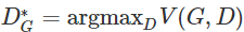
Given a generator G, which represents the correct identification of real and fake data points by the discriminator D. The optimal discriminator obtained from the above equation can be expressed as  (denoted as D_G* below). The value function is defined as:

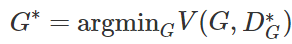
We can then formulate the optimization problem as:
Now G’s objective has reversed; when D=D_G*, the optimal G minimizes the previous equation. In the paper, the authors prefer to solve the optimization value functions of G and D to solve the minimax game:

For D, the goal is to maximize the formula (strong recognition capability), while for G, it aims to minimize (the generated data approaches actual data). The entire training process is an iterative process. In fact, the minimax game can be understood separately, that is, first maximizing V(D,G) given G to obtain D, then fixing D and minimizing V(D,G) to obtain G. Among them, maximizing V(D,G) given G evaluates the difference or distance between P_G and P_data.
Finally, we can express the optimization problem as:
The above provides the formal expression of the GAN concept and optimization process. Through these expressions, we can understand the basic process and optimization methods of the entire generative adversarial network. Of course, with these concepts, we can directly find a segment of GAN code on GitHub, make some modifications, and run it well. But if we want to understand GAN more thoroughly and comprehensively, we still need to know many derivation processes. For example, when D can maximize the value function V(D,G), what kind of neural networks (or functions) should D and G use, and what loss functions they need, etc. In short, there are many theoretical details and derivation processes that we need to further explore.
Theoretical Derivation
In the original GAN paper, the method for measuring the difference or distance between the generative distribution and the real distribution is the JS divergence, and the JS divergence is constructed using KL divergence during the derivation of the training process. Therefore, this part will start from the theoretical foundation and further derive the conditions that the optimal discriminator and generator need to satisfy. Finally, we will use the derivation results to mathematically restate the training process. This part provides strong theoretical support for our understanding of the specific implementation in the next part.
KL Divergence
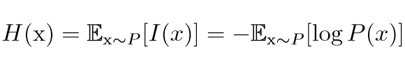
In information theory, we can use Shannon entropy to quantify the total uncertainty in a probability distribution:
If we have two separate probability distributions P(x) and Q(x) for the same random variable x, we can use KL divergence (Kullback-Leibler divergence) to measure the difference between these two distributions:
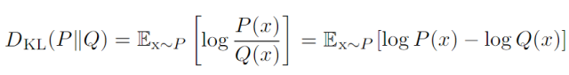
In the case of discrete variables, KL divergence measures the additional amount of information needed when we send a message containing symbols generated by probability distribution P, using a code designed to minimize the length of messages produced by probability distribution Q.
KL divergence has many useful properties, the most important of which is that it is non-negative. KL divergence is 0 if and only if P and Q are the same distribution in the case of discrete variables, or “almost everywhere” the same in the case of continuous variables. Because KL divergence is non-negative and measures the difference between two distributions, it is often used as a kind of distance between distributions. However, it is not truly a distance because it is not symmetric: for some P and Q, D_KL(P||Q) is not equal to D_KL(Q||P). This asymmetry means that choosing D_KL(P||Q) or D_KL(Q||P) has a significant impact.
In Li Hongyi’s explanation, KL divergence can be derived from maximum likelihood estimation. Given a sample data distribution P_data(x) and a generated data distribution P_G(x;θ), GAN hopes to find a set of parameters θ that minimizes the distance between distributions P_g(x;θ) and P_data(x), which means finding a set of generator parameters that allows the generator to produce very realistic images.
Now we can extract a set of real images from the training set to train the parameters θ in the distribution P_G(x;θ) to approximate the real distribution. Thus, we can extract m real samples {x^1,x^2,…,x^𝑚} from P_data(x), where the symbol “^” represents the exponent, that is, the i-th sample in x. For each real sample, we can calculate P_G(x^i;θ), that is, the probability of sample x^i appearing in the generated distribution determined by θ. Therefore, we can construct the likelihood function:

Where “∏” represents multiplication, and P_G(x^i;θ) represents the probability of the i-th sample appearing in the generated distribution. From this likelihood function, we know that the probability of the m real samples all appearing in the P_G(x;θ) distribution is expressed as L. Because if the P_G(x;θ) distribution is similar to the P_data(x) distribution, the real data is likely to appear in the P_G(x;θ) distribution, thus the probability of all m samples appearing in the P_G(x;θ) distribution will be very high.
We can now maximize the likelihood function L to obtain the generated distribution (i.e., the optimal parameters θ) closest to the real distribution:
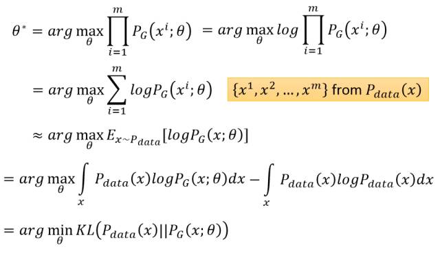
In the above derivation, we want to maximize the likelihood function L. If we take the logarithm of the likelihood function, the multiplication “∏” can be transformed into addition “∑”, and this process does not change the optimization result. Therefore, we can transform the maximum likelihood estimation into finding the parameters θ that maximize E[logP_G(x;θ)], and the expectation E[logP_G(x;θ)] can be expanded into an integral form over x: ∫P_data(x)logP_G(x;θ)dx. Since this optimization process is for θ, adding an integral that does not contain θ does not affect the optimization effect, that is, we can add -∫P_data(x)logP_data(x)dx. After adding this integral, we can combine the two integrals and construct a form similar to KL divergence. The process is as follows:
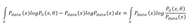
This integral is the integral form of KL divergence, so if we need to find the parameters θ that make the generated distribution P_G(x;θ) as close as possible to the real distribution P_data(x), we only need to find the parameters θ that minimize KL divergence. If the optimal parameters θ are obtained, the images generated by the generator will appear very realistic.
Problems in Derivation
Next, we must prove that this optimization problem has a unique solution G*, and that this unique solution satisfies P_G=P_data. However, before starting to derive the optimal discriminator and optimal generator, we need to understand Scott Rome’s views on the derivation in the original paper, as he believes that the original paper overlooked the invertibility condition, thus the derivation of the optimal solution is not perfect.
In the original GAN paper, there is a thought that differs from many other methods, namely that the generator G does not need to satisfy the invertibility condition. Scott Rome believes this point is very important because, in practice, G is non-invertible. Many proof notes overlook this point, and they mistakenly used the integral change of variables formula in their proof, which is based on the invertibility condition of G. Scott believes that the proof can only be based on the validity of the following equation:

This equation comes from the Radon-Nikodym theorem in measure theory, which is expressed in Proposition 1 of the original paper as follows:
We see that the lecture uses the integral change of variables formula, but performing the change of variables requires calculating G^(-1), and the inverse of G is not assumed to exist. Moreover, in practice with neural networks, it does not exist. Perhaps this method is too common in machine learning and statistical literature, so we overlooked it.
Optimal Discriminator
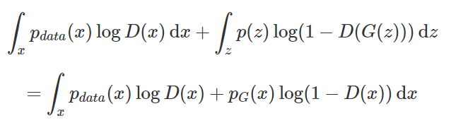
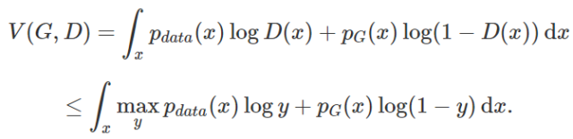
In the first step of the minimax game, given the generator G, maximize V(D,G) to obtain the optimal discriminator D. Among them, maximizing V(D,G) evaluates the difference or distance between P_G and P_data. Because in the original paper, the value function can be written as an integral over x, i.e., expanding the mathematical expectation into an integral form:
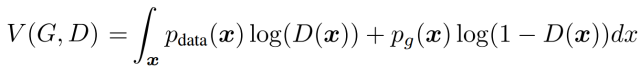
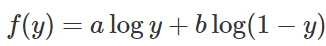
Actually, finding the maximum value of the integral can be transformed into finding the maximum value of the integrand. The purpose of finding the maximum value of the integrand is to obtain the optimal discriminator D, so any terms not involving the discriminator can be considered constant terms. As shown, both P_data(x) and P_G(x) are scalars, so the integrand can be expressed as a*D(x)+b*log(1-D(x)).
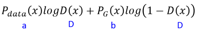
If we let D(x) equal y, the integrand can be written as:
To find the optimal extreme point, if a+b≠0, we can use the following first derivative to solve:
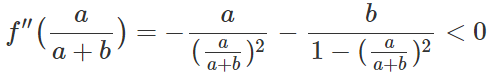
Where a,b∈(0,1). Since the first derivative equals zero and the second derivative is less than zero, we know that a/(a+b) is the maximum value. If we substitute a=P_data(x), b=P_G(x) into this extreme value, then the optimal discriminator D(x)=P_data(x)/(P_data(x)+P_G(x)).
Finally, we can write the expression of the value function as:
If we let D(x)=P_data/(P_data+P_G), then we can maximize the value function V(G,D). Since f(y) has a unique maximum value in its domain, the optimal D is also unique, and no other D can achieve the maximum value.
In fact, this optimal D is not computable in practice, but it is mathematically important. We do not know the prior P_data(x), so we will never use it in training. On the other hand, its existence allows us to prove that the optimal G exists, and in training, we only need to approximate D.
Optimal Generator
Of course, the goal of the GAN process is to make P_G=P_data. What does this mean for the optimal D? We can substitute this equality into the expression of D_G*:
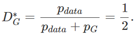
This means that the discriminator is completely confused; it cannot distinguish between P_data and P_G, that is, the probability of judging that the sample comes from P_data and P_G is both 1/2. Based on this perspective, the authors of GAN proved that G is the solution to the minimax game. The theorem is as follows:
“If and only if P_G=P_data, the global minimum point of the training standard C(G)=maxV(G,D) can be reached.”
The above theorem is the second step of the minimax game, seeking the generator G that minimizes V(G,D*) (where G* represents the optimal discriminator). The reason that P_G(x)=P_data(x) can minimize the value function is that at this point, the JS divergence [JSD(P_data(x) || P_G(x))] equals zero. The detailed explanation of this process is as follows.
The original paper’s theorem is a “if and only if” statement, so we need to prove it from both directions. First, we will prove the value of C(G) from the reverse approach and then use the new knowledge obtained from the reverse to prove it from the forward approach. Let P_G=P_data (the reverse means we know the optimal condition in advance and do the derivation), we can derive backwards:
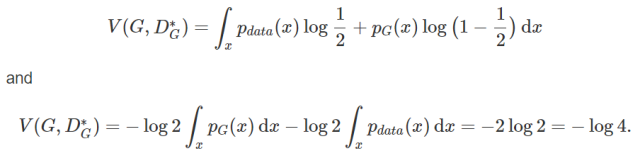
That value is a candidate for the global minimum because it only occurs when P_G=P_data. We now need to prove from the forward that this value is often the minimum, that is, to satisfy the conditions of “when” and “only when” at the same time. Now abandoning the assumption of P_G=P_data, for any G, we can substitute the optimal discriminator D* obtained in the previous step into C(G)=maxV(G,D) as follows:

Because it is known that -log4 is the global minimum candidate, we want to construct a value to make log2 appear in the equation. Therefore, we can add or subtract log2 to each integral, multiplying by the probability density. This is a very common mathematical proof technique that does not change the equation, because essentially we are just adding 0 to the equation.

Using this technique is mainly to hope to construct a form that includes log2 and JS divergence. The simplified expression can be obtained as follows: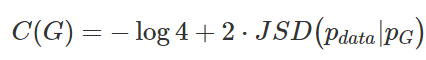
This divergence is actually the square of the Jenson-Shannon distance metric. According to its properties: when P_G=P_data, JSD(P_data||P_G) equals 0. In summary, the generated distribution can only achieve the optimal generator when it equals the real data distribution.
Convergence
Now, the main part of the paper has been proven: that is, P_G=P_data is the optimal point of maxV(G,D). In addition, the original paper also has additional proofs indicating that given sufficient training data and the correct environment, the training process will converge to the optimal G, which we will not discuss in detail.
Restating the Training Process
Below is the final step of the derivation, where we will restate the entire parameter optimization process and briefly introduce the various processes involved in actual training.
-
Parameter Optimization Process:
If we need to find the optimal generator, then given a discriminator D, we can treat maxV(G,D) as the loss function L(G) for training the generator. Since we have set the loss function, we can use optimization algorithms such as SGD, Adam, etc., to update the parameters of the generator G. The gradient descent parameter optimization process is as follows:
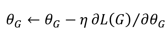
Where finding the partial derivative of L(G) with respect to θ_G involves finding the partial derivative of max{V(G,D)}. This method of differentiating the max function exists and is usable.
Now given an initial G_0, we need to find D_0* that maximizes V(G_0,D), so the process of updating the discriminator can also be viewed as a training process with a loss function of -V(G,D).
And from the previous derivation, we know that V(G,D) is actually just a constant term away from the JS divergence between distributions P_data(x) and P_G(x). Therefore, this iterative adversarial process can be expressed as:
-
Given G_0, maximize V(G_0,D) to obtain D_0*, that is, max[JSD(P_data(x)||P_G0(x)];
-
Fix D_0*, calculate θ_G1 ← θ_G0 −η(dV(G,D_0*) /dθ_G) to obtain the updated G_1;
-
Fix G_1, maximize V(G_1,D_0*) to obtain D_1*, that is, max[JSD(P_data(x)||P_G1(x)];
-
Fix D_1*, calculate θ_G2 ← θ_G1 −η(dV(G,D_0*) /dθ_G) to obtain the updated G_2;
-
…
-
Actual Training Process:
According to the definition of the value function V(G,D), we need to find two mathematical expectations, namely E[log(D(x))] and E[log(1-D(G(z)))], where x follows the real data distribution and z follows the initialization distribution. However, in practice, we cannot use integrals to obtain these two mathematical expectations, so generally we can sample from infinite real data and infinite generators to approximate the real mathematical expectations.
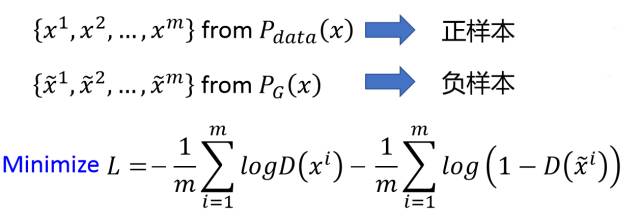
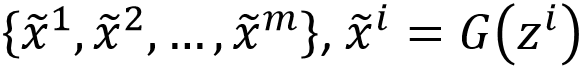
Now, given the generator G and hoping to calculate maxV(G,D) to obtain the discriminator D, we first need to sample m samples {x^1,x^2,…,x^m} from P_data(x), and sample m samples from the generator P_G(x):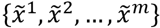 . Therefore, maximizing the value function V(G,D) can be approximated using the following expression:
If we need to calculate the aforementioned maximization process, we can use an equivalent form of training method. If we have a binary classifier D (parameterized by θ_d), then of course this classifier can be a deep neural network, and the output of the maximization process will be the output of this classifier D(x). Now we sample real samples from P_data(x) as positive samples and sample negative samples from P_G(x), while using the function that approximates negative V(G,D) as the loss function. Thus, we express it as a standard binary classifier training process:
In practice, we must use iterative and numerical calculation methods to implement the minimax game process. It is not computationally feasible to fully optimize D in the internal loop of training, and a limited dataset can also lead to overfitting. Therefore, we can alternate between k optimization steps for D and one optimization step for G. Thus, we only need to slowly update G, and D will always stay near the optimal solution, a strategy similar to SML/PCD training.
In summary, we can describe the entire training process. For each iteration:
-
Extract m samples from the real data distribution P_data
-
Extract m noise samples from the prior distribution P_prior(z)
-
Feed the noise samples into G to generate data
 , and update the discriminator parameters θ_d by maximizing the approximation of V, that is, maximizing
 , and the update iteration formula for the discriminator parameters is
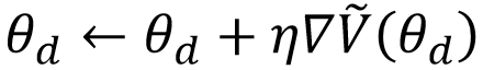
This is the process of learning the discriminator D. Since the process of learning D is the process of calculating JS divergence, and we hope to maximize the value function, this step will be repeated k times.
-
Extract another m noise samples {z^1,…,z^m} from the prior distribution P_prior(z)
-
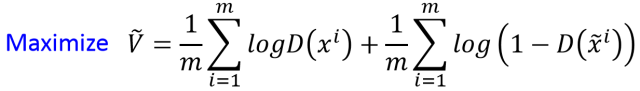
Update the generator parameters θ_g by minimizing V^tilde, that is, maximizing
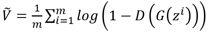 , and the update iteration formula for the generator parameters is
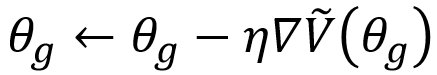
The above is the process of learning the generator parameters. This process will only occur once in an iteration to avoid excessive updates that cause the JS divergence to rise.
Implementation
In the previous issue of Machine Heart’s GitHub project, we implemented a simple CNN from scratch using TensorFlow. We not only introduced the basic operations of TensorFlow but also implemented LeNet-5 starting from a fully connected neural network. In the first GitHub implementation, we uploaded three segments of implementation code. The second upload supplemented the fully connected network for MNIST image recognition, and we annotated all the code of this model line by line. The third upload supplemented the construction of a simple CNN using Keras, and we also added a lot of comments. This article is the second GitHub implementation, and first provides the GAN implementation code and comments, and then we will combine the above theoretical analysis with the implementation code and display it in Jupyter Notebook. Although the first implementation used a relatively simple high-level API (Keras), we will later supplement the code and comments for building GAN with TensorFlow.
GitHub implementation address:
https://github.com/jiqizhixin/ML-Tutorial-Experiment
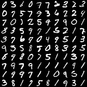
Machine Heart first implemented this generative adversarial network based on Keras with a TensorFlow backend, and we trained the model on the MNIST dataset to generate a series of handwritten fonts. This chapter only briefly explains part of the implementation code, for more complete and detailed annotations, please check the GitHub project address.
Generative Model
First, we need to define a generator G that transforms the input random noise into images. Below is the defined generative model, which first inputs a vector of 100 elements, randomly generated from a certain distribution. Then, it uses two fully connected layers to expand this input vector to 1024 dimensions and 128*7*7 dimensions, after which it starts reshaping the one-dimensional tensor produced by the fully connected layers into a two-dimensional tensor, i.e., a grayscale image in MNIST. We note that the activation function used in this model is tanh, so we also tried converting it to the relu function, but found that if the generative model was converted to the relu function, its output would become a gray image.
The data transmitted through the fully connected layers will pass through several upsampling layers and convolutional layers. We note that the convolution kernel used in the last convolutional layer is 1, so the image generated after the last convolutional layer is a two-dimensional grayscale image. For more detailed analysis, please check the Machine Heart GitHub project.
def generator_model():
    # Build the architecture of the generator, first import the sequential model (sequential), i.e., the linear stacking of multiple network layers
    model = Sequential()
    # Add a fully connected layer, input is 100-dimensional vector, output is 1024-dimensional
    model.add(Dense(input_dim=100, output_dim=1024))
    # Add an activation function tanh
    model.add(Activation('tanh'))
    # Add a fully connected layer, output is 128×7×7 dimensions
    model.add(Dense(128*7*7))
    # Add a batch normalization layer, which re-normalizes the activation values of the previous layer on each batch, making its output data mean close to 0 and standard deviation close to 1
    model.add(BatchNormalization())
    model.add(Activation('tanh'))
    # Reshape layer is used to convert the input shape into a specific shape, turning the vector containing 128*7*7 elements into a 7×7×128 tensor
    model.add(Reshape((7, 7, 128), input_shape=(128*7*7,)))
    # 2D upsampling layer, which repeats the rows and columns of the data 2 times respectively
    model.add(UpSampling2D(size=(2, 2)))
    # Add a 2D convolutional layer, kernel size is 5×5, activation function is tanh, a total of 64 convolution kernels, using padding to keep the image size unchanged
    model.add(Conv2D(64, (5, 5), padding='same'))
    model.add(Activation('tanh'))
    model.add(UpSampling2D(size=(2, 2)))
    # Set the convolution kernel to 1 to output the image dimension
    model.add(Conv2D(1, (5, 5), padding='same'))
    model.add(Activation('tanh'))
    return model
Concatenation
The generative model defined above is capable of generating images G(z;θ_g), and when training the generative model, we need to fix the discriminator D to minimize the value function and seek a better generative model. This means we need to concatenate the generative model and the discriminative model together, fixing the weights of D to train the weights of G. The following defines this process, where we first add the previously defined generative model, then concatenate the defined discriminative model below the generative model, and we set the discriminative model as non-trainable. Thus, training this combined model can effectively update the parameters of the generative model.
def generator_containing_discriminator(g, d):
    # Concatenate the previously defined generator architecture and discriminator architecture into a larger neural network, used to discriminate the generated images
    model = Sequential()
    # First add the generator architecture, then make d non-trainable, i.e., fix d
    # Therefore, train the generator under the condition of given d, i.e., optimize the generator by feeding the generated results into the discriminator for identification
    model.add(g)
    d.trainable = False
    model.add(d)
    return model
Discriminative Model
The discriminative model is relatively traditional for image recognition models. We can use several convolutional layers and max-pooling layers according to classic methods, and then flatten into a one-dimensional tensor and use several fully connected layers as the architecture. We tried replacing the tanh activation function with the relu activation function, but found no significant changes in the first two epochs.
def discriminator_model():
    # Below builds the architecture of the discriminator, also using a sequential model
    model = Sequential()
    # Add a 2D convolutional layer, kernel size is 5×5, activation function is tanh, input shape in 'channels_first' mode is (samples,channels,rows,cols)
    # In 'channels_last' mode it is (samples,rows,cols,channels), output is 64 dimensions
    model.add(
            Conv2D(64, (5, 5),
            padding='same',
            input_shape=(28, 28, 1))
            )
    model.add(Activation('tanh'))
    # Apply max pooling to the spatial signal, pool_size of (2,2) represents reducing the image to half its original length in both dimensions
    model.add(MaxPooling2D(pool_size=(2, 2)))
    model.add(Conv2D(128, (5, 5)))
    model.add(Activation('tanh'))
    model.add(MaxPooling2D(pool_size=(2, 2)))
    # Flatten layer converts multi-dimensional input to one dimension, commonly used in transitioning from convolutional layers to fully connected layers
    model.add(Flatten())
    model.add(Dense(1024))
    model.add(Activation('tanh'))
    # A node for binary classification, and use the output of the sigmoid function as the concept
    model.add(Dense(1))
    model.add(Activation('sigmoid'))
    return model
Training
The training part is relatively long and worth discussing in detail. In summary, the following training process can be described as:
-
Load MNIST data
-
Split the data into training and testing sets and assign them to variables
-
Set hyperparameters for the training model
-
Compile the training process of the model
-
In each iteration, extract generated images and real images and label them
-
Then input the data into the discriminative model, and perform training and calculate losses
-
Fix the discriminative model, train the generative model, and calculate losses, finishing this iteration
The above is a brief introduction to the training process, and we will showcase a more detailed analysis on GitHub in combination with the theoretical derivation above.
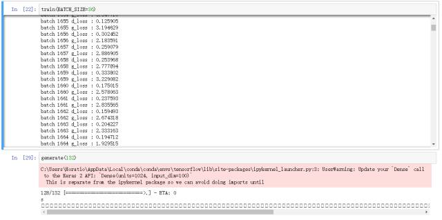
def train(BATCH_SIZE):
    # It seems that we cannot directly import the dataset in China. We tried several times without success, later we downloaded the dataset to the local '~/.keras/datasets/', which is the .keras folder in the current directory (mine is under the user folder).
    # The download address is: https://s3.amazonaws.com/img-datasets/mnist.npz
    (X_train, y_train), (X_test, y_test) = mnist.load_data()
    # image_data_format chooses "channels_last" or "channels_first", this option specifies the order of dimensions Keras will use.
    # "channels_first" assumes the order of dimensions for 2D data is (channels, rows, cols), for 3D data it is (channels, conv_dim1, conv_dim2, conv_dim3)
    # Convert field types and import the data into variables
    X_train = (X_train.astype(np.float32) - 127.5)/127.5
    X_train = X_train[:, :, :, None]
    X_test = X_test[:, :, :, None]
    # X_train = X_train.reshape((X_train.shape, 1) + X_train.shape[1:])
    # Assign the defined model architecture to specific variables
    d = discriminator_model()
    g = generator_model()
    d_on_g = generator_containing_discriminator(g, d)
    # Define the optimization algorithm and hyperparameters used for updating the generator model discriminator model
    d_optim = SGD(lr=0.001, momentum=0.9, nesterov=True)
    g_optim = SGD(lr=0.001, momentum=0.9, nesterov=True)
    # Compile the three neural networks and set the loss functions and optimization algorithms, where the loss functions are all binary classification cross-entropy functions. Compilation is used to configure the learning process of the model
    g.compile(loss='binary_crossentropy', optimizer="SGD")
    d_on_g.compile(loss='binary_crossentropy', optimizer=g_optim)
    # Before the previous architecture trains the generator, it is necessary to first set the discriminator as trainable.
    d.trainable = True
    d.compile(loss='binary_crossentropy', optimizer=d_optim)
    # Below, training is conducted under the condition of satisfying epoch
    for epoch in range(30):
        print("Epoch is", epoch)
        # Calculate the number of iterations required for one epoch, that is, the number of training samples divided by the batch size; where shape[0] reads the length of the first dimension of the matrix
        print("Number of batches", int(X_train.shape[0]/BATCH_SIZE))
        # In one epoch, perform iterative training
        for index in range(int(X_train.shape[0]/BATCH_SIZE)):
            # Randomly generated noise follows a uniform distribution, with a lower bound of -1 and an upper bound of 1, outputting BATCH_SIZE×100 samples; that is, extracting a batch of random samples
            noise = np.random.uniform(-1, 1, size=(BATCH_SIZE, 100))
            # Extract a batch of real images
            image_batch = X_train[index*BATCH_SIZE:(index+1)*BATCH_SIZE]
            # The generated images use the generator to infer the random noise; verbose is the log display, 0 means not outputting log information to the standard output, 1 means outputting progress bar records
            generated_images = g.predict(noise, verbose=0)
            # Output a generated image every 100 iterations
            if index % 100 == 0:
                image = combine_images(generated_images)
                image = image*127.5+127.5
                Image.fromarray(image.astype(np.uint8)).save(
                    "./GAN/"+str(epoch)+"_"+str(index)+".png")
            # Concatenate real images and generated images into a multi-dimensional array; real images on top, generated images on the bottom
            X = np.concatenate((image_batch, generated_images))
            # Generate labels for images, that is, a list containing twice the batch size; the first batch size is all 1, representing real images, the second batch size is all 0, representing fake images
            y = [1] * BATCH_SIZE + [0] * BATCH_SIZE
            # Loss of the discriminator; perform one parameter update on a batch of data
            d_loss = d.train_on_batch(X, y)
            print("batch %d d_loss : %f" % (index, d_loss))
            # Randomly generated noise follows a uniform distribution
            noise = np.random.uniform(-1, 1, (BATCH_SIZE, 100))
            # Fix the discriminator
            d.trainable = False
            # Calculate the loss of the generator; perform one parameter update on a batch of data
            g_loss = d_on_g.train_on_batch(noise, [1] * BATCH_SIZE)
            # Make the discriminator trainable again
            d.trainable = True
            print("batch %d g_loss : %f" % (index, g_loss))
            # Save the weights of the generator and discriminator every 100 iterations
            if index % 100 == 9:
                g.save_weights('generator', True)
                d.save_weights('discriminator', True)
Experiment
In practice, after training for 30 epochs, we can obtain the following good generation results:
Of course, we also encountered many training issues, such as learning rate, batch size, activation functions, etc. The learning rate is generally set between 0.001 and 0.0005, and there are many other learning rates that have not been tested. We used relatively small batch sizes, such as 16, 32, 64, etc. A smaller learning rate may not require as many training epochs. We found that if the activation function of the generative model is modified to relu, the generated image is likely to appear as a gray image, and the training losses of the generative model and discriminator may behave as follows:
 #batch_size=32
batch 2000 d_loss : 0.000318
batch 2000 g_loss : 7.618911
In the above case, after 2000 iterations, the loss of the discriminator kept decreasing while the loss of the generator kept increasing. Under normal circumstances, I found that the losses of the generator and discriminator would alternate between rising and falling within a certain range, and the training loss situation after 2000 iterations was:
 #batch_size=36
batch 2000 g_loss : 1.663281
batch 2000 d_loss : 0.483616
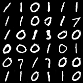
In addition, we also found many problematic generation patterns, such as the following generated results tending more towards 0 and 1:
Finally, here is our training completion marker.
References:
Original GAN paper:
https://arxiv.org/pdf/1406.2661.pdf
Goodfellow NIPS 2016 Tutorial: https://arxiv.org/abs/1701.00160
Li Hongyi MLDS17: http://speech.ee.ntu.edu.tw/~tlkagk/courses_MLDS17.html
Scott Rome GAN Derivation:
http://srome.github.io//An-Annotated-Proof-of-Generative-Adversarial-Networks-with-Implementation-Notes/
