MLNLP community is a well-known machine learning and natural language processing community both domestically and internationally, covering NLP master’s and doctoral students, university teachers, and corporate researchers.The vision of the community is to promote communication and progress between the academic and industrial circles of natural language processing and machine learning, especially for beginners. Reprinted from | PaperWeekly Author | Song Xun Institution | Nanjing University Research Direction | Data Mining

We first clarify the relationship between single-hidden-layer neural networks and Gaussian processes (GP), then extend the concept to multi-hidden-layer neural networks, and finally discuss how to use GP to perform traditional neural network tasks, namely learning and prediction.

1

『Single Hidden Layer Neural Networks and NNGP』

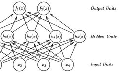
In the fully connected neural network shown in the figure below:

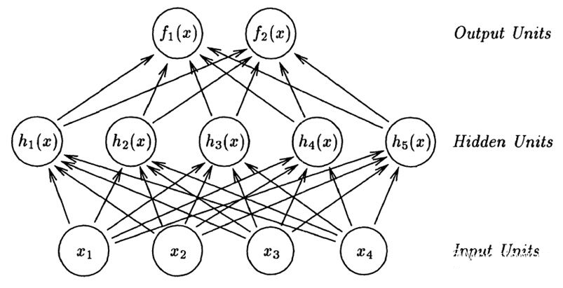
The output of the function can be written as:

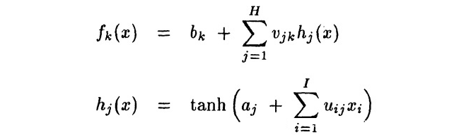
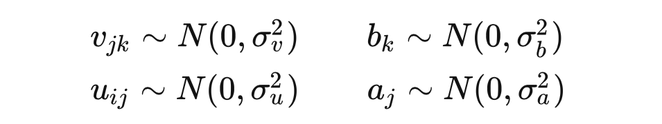
We assume that all parameters of the network follow a Gaussian distribution:

Now we study the value of the th output unit under some input , that is, .Because , for any , the expected value of the output of the th hidden unit is 0: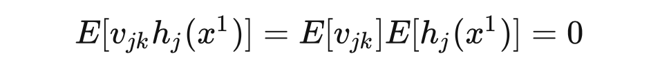The variance of the output of the th hidden unit is:Note that for all , the value of is the same (because it only depends on , , and ), so we set .Since all hidden layer outputs are independent and identically distributed, by the Central Limit Theorem, we know that as approaches infinity, follows a Gaussian distribution with variance . Therefore, when approaches infinity, we obtain the prior distribution of as: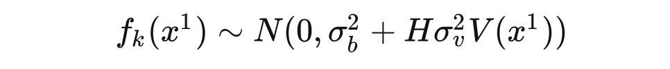To limit the variance of from approaching infinity, for some fixed , we set , yielding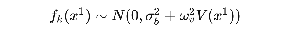Now for a set of inputs , we consider their corresponding output joint probability distribution. By definition, should follow a multivariate Gaussian distribution with a mean of 0, where the covariance between any two outputs and is defined as:where is equal for all .At this point, we say that constitutes a Gaussian process, and the definition of a Gaussian process is:

Definition: A Gaussian process is a collection of random variables, any finite number of which have a joint Gaussian distribution.

In fact, rather than saying that the Gaussian process describes these variables, it is more accurate to say that it describes the distribution of a function:For any number of inputs, the corresponding joint probability distribution of the function outputs is a multivariate Gaussian distribution.[1] The authors in conducted the following experiments to validate this Gaussian distribution: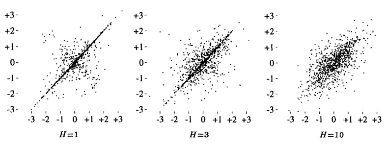The parameters are set as: . In the above three figures, the hidden layer width is set to 1, 3, and 10, respectively.Each point represents a sample of the network parameters (i.e., each point is a separate neural network), with the x-axis and y-axis representing the function outputs when the inputs are and .It can be seen that as gradually increases, the two outputs exhibit a bivariate Gaussian distribution (with a clear correlation).Now let’s intuitively understand the significance of this conclusion.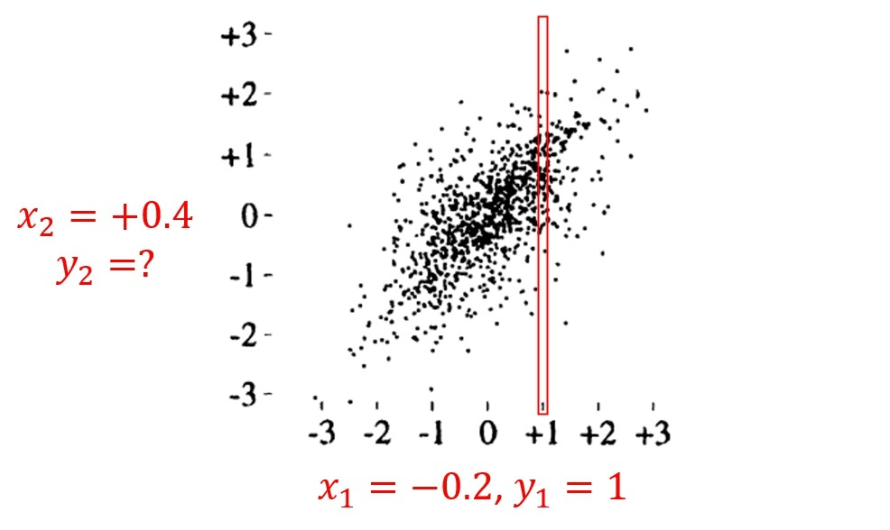Taking the situation with as an example. Still those two inputs, one and one . Now we assume that the label of is known:, then what should the label of be?Without the label of , we do not know which points in the graph (representing neural networks) can fit the relationship between and . However, once we know , we can at least narrow down the selection range to the red box in the above graph, as only the models within it can predict in accordance with our observed values. At this point, one feasible approach is to consider the predictions of all models within the box for and provide a final output (e.g., taking their mean).In this example, ( ) is equivalent totraining samples, while isthe test set.

2

『Multi-Hidden Layer Neural Networks and NNGP』

We already know that each dimension of output from a single hidden layer neural network can be viewed as a Gaussian process (GP), and this conclusion can be extended tomulti-hidden fully connected neural networks [3].For input , let the output of the th unit in the layer be denoted as , and the computation of the neural network can be represented as: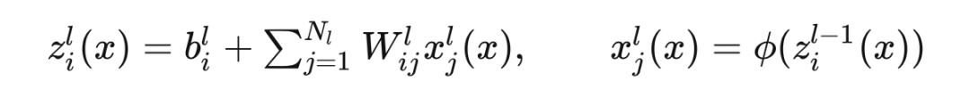where is the activation function.For input , its output is a Gaussian process (similar to the principle of single hidden layer):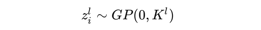where is called the kernel, and its recursive formula is: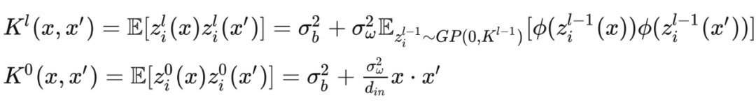It can be seen that the only nonlinear part in the entire recursive formula is the activation function . This prevents us from obtaining a complete analytical formula. Fortunately, for some specific activation functions, equivalent analytical expressions can be derived. For example, for the commonly used ReLU function, the recursive formula can be expressed in the following analytical form:

3

『Making Predictions with NNGP』

Before discussing the prediction methods of NNGP, we need to lay down a foundational knowledge:Conditional Probability Distribution of Multivariate Gaussian Distribution.Consider a vector that follows a Gaussian distribution, we divide it into two parts: and . Then we have: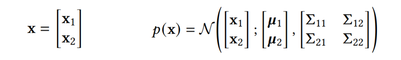Given the known , the distribution of can be expressed as:where: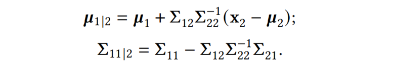Note that is the distribution of when is known. Unlike , which is theprior distribution, is aposterior distribution, which utilizes the observed values of and the covariance between and , eliminating some uncertainty of the original .Now we know how to make predictions with NNGP:Recall that our conclusions from the previous two sections were:For fully connected layer neural networks, when the network parameters follow a Gaussian distribution and the hidden layer width is sufficiently large, each dimension of output is a Gaussian process.As with conventional learning problems, our dataset consists of two parts:the training set and the test set.The training set consists of each sample including an input value and an observed value: while the test set only has input samples We denote them in vector form: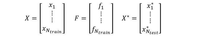We are interested in the unknown quantity , and according to our conclusions, the joint Gaussian probability distribution for and is: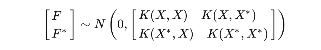Now that we know , the posterior distribution of is:

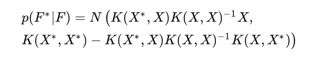
4

『Summary』

The biggest difference between traditional neural networks and Neural Network Gaussian Processes (NNGP) is that the latter does not havean explicit training process (i.e., adjusting parameters through BP), but only leverages the structural information of the neural network (including the distribution of network parameters and activation functions) to generate a kernel, i.e., covariance matrix.We don’t even need to actually generate a neural network to obtain the kernel:Assuming we use the ReLU activation function, then from: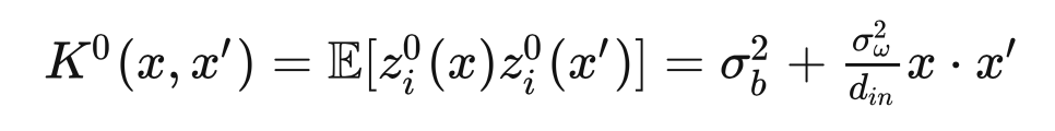to the recursive formula: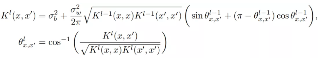we do not need to involve the specific parameters of the neural network.In addition, we can directly specify an empirical covariance matrix, such assquared exponential error: 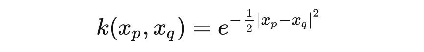The farther apart and are, the smaller the covariance, and vice versa. This is intuitive because for acontinuous and smoothing function, points that are closer together will always have stronger correlations—this is also the consensus on which the empirical covariance function relies.References[1] Neal R M. Bayesian learning for neural networks[M]. Springer Science & Business Media, 2012.[2] Williams C K I, Rasmussen C E. Gaussian processes for machine learning[M]. Cambridge, MA: MIT press, 2006.[3] Lee J, Bahri Y, Novak R, et al. Deep neural networks as Gaussian processes[J]. arXiv preprint arXiv:1711.00165, 2017.[4] Roman Garnett. BAYESIAN OPTIMIZATION.Technical Group Chat Invitation

△Press and hold to add the assistant

Scan the QR code to add the assistant’s WeChat

Please note: Name-School/Company-Research Direction(e.g., Xiao Zhang-Harbin Institute of Technology-Dialogue System) to apply to join the Natural Language Processing/Pytorch and other technical group chats

About Us

MLNLP community is a grassroots academic community jointly established by domestic and foreign scholars in machine learning and natural language processing, which has now developed into a well-known machine learning and natural language processing community both domestically and internationally, aimed at promoting progress between the academic and industrial circles of machine learning and natural language processing and enthusiasts.The community can provide an open communication platform for related practitioners’ further education, employment, and research. Everyone is welcome to follow and join us.