
Click the above “Beginner Learning Vision” to choose to add Star or “Pin”
Important content delivered in real-time
-
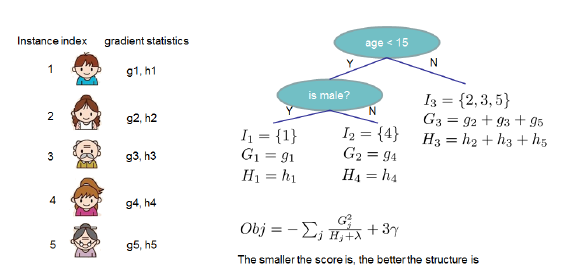
: The sum of the first-order partial derivatives of the samples contained in the leaf node is a constant; -
: The sum of the second-order partial derivatives of the samples contained in the leaf node is a constant;

class XGBoostTree(Tree):    # Node splitting    def _split(self, y):        col = int(np.shape(y)[1]/2)        y, y_pred = y[:, :col], y[:, col:]        return y, y_pred
    # Information gain calculation formula    def _gain(self, y, y_pred):        Gradient = np.power((y * self.loss.gradient(y, y_pred)).sum(), 2)        Hessian = self.loss.hess(y, y_pred).sum()        return 0.5 * (Gradient / Hessian)
    # Tree splitting gain calculation    def _gain_by_taylor(self, y, y1, y2):        # Node splitting        y, y_pred = self._split(y)        y1, y1_pred = self._split(y1)        y2, y2_pred = self._split(y2)
        true_gain = self._gain(y1, y1_pred)        false_gain = self._gain(y2, y2_pred)        gain = self._gain(y, y_pred)        return true_gain + false_gain - gain
    # Optimal weight for leaf nodes    def _approximate_update(self, y):        # y split into y, y_pred        y, y_pred = self._split(y)        # Newton's Method        gradient = np.sum(y * self.loss.gradient(y, y_pred), axis=0)        hessian = np.sum(self.loss.hess(y, y_pred), axis=0)        update_approximation =  gradient / hessian
        return update_approximation
# Tree fitting method def fit(self, X, y): self._impurity_calculation = self._gain_by_taylor self._leaf_value_calculation = self._approximate_update super(XGBoostTree, self).fit(X, y)class XGBoost(object):
def __init__(self, n_estimators=200, learning_rate=0.001, min_samples_split=2, min_impurity=1e-7, max_depth=2): self.n_estimators = n_estimators # Number of trees self.learning_rate = learning_rate # Step size for weight update self.min_samples_split = min_samples_split # The minimum n of sampels to justify split self.min_impurity = min_impurity # Minimum variance reduction to continue self.max_depth = max_depth # Maximum depth for tree
# Cross-entropy loss self.loss = LogisticLoss()
# Initialize model self.estimators = [] # Forward stepwise training for _ in range(n_estimators): tree = XGBoostTree( min_samples_split=self.min_samples_split, min_impurity=min_impurity, max_depth=self.max_depth, loss=self.loss)
self.estimators.append(tree)
def fit(self, X, y): y = to_categorical(y)
y_pred = np.zeros(np.shape(y)) for i in range(self.n_estimators): tree = self.trees[i] y_and_pred = np.concatenate((y, y_pred), axis=1) tree.fit(X, y_and_pred) update_pred = tree.predict(X) y_pred -= np.multiply(self.learning_rate, update_pred)
def predict(self, X): y_pred = None # Prediction for tree in self.estimators: update_pred = tree.predict(X) if y_pred is None: y_pred = np.zeros_like(update_pred) y_pred -= np.multiply(self.learning_rate, update_pred)
y_pred = np.exp(y_pred) / np.sum(np.exp(y_pred), axis=1, keepdims=True) # Convert probability predictions to labels y_pred = np.argmax(y_pred, axis=1) return y_predfrom sklearn import datasets
data = datasets.load_iris()
X = data.data
y = data.target
X_train, X_test, y_train, y_test = train_test_split(X, y, test_size=0.4, seed=2)
clf = XGBoost()
clf.fit(X_train, y_train)
y_pred = clf.predict(X_test)
accuracy = accuracy_score(y_test, y_pred)
print ("Accuracy:", accuracy)Accuracy: 0.9666666666666667pip install xgboostimport xgboost as xgb
from xgboost import plot_importance
from matplotlib import pyplot as plt
# Set model parameters
params = { 'booster': 'gbtree', 'objective': 'multi:softmax', 'num_class': 3, 'gamma': 0.1, 'max_depth': 2, 'lambda': 2, 'subsample': 0.7, 'colsample_bytree': 0.7, 'min_child_weight': 3, 'silent': 1, 'eta': 0.001, 'seed': 1000, 'nthread': 4,}
plst = params.items()
dtrain = xgb.DMatrix(X_train, y_train)
num_rounds = 200
model = xgb.train(plst, dtrain, num_rounds)
# Predict on the test set
dtest = xgb.DMatrix(X_test)
y_pred = model.predict(dtest)
# Calculate accuracy
accuracy = accuracy_score(y_test, y_pred)
print ("Accuracy:", accuracy)
# Plot feature importance
plot_importance(model)
plt.show();Accuracy: 0.9166666666666666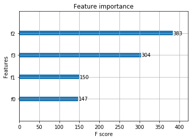
Good news!
Beginner Learning Vision Knowledge Circle
Is now open to the public👇👇👇
Download 1: OpenCV-Contrib Extension Module Chinese Version Tutorial
Reply in the "Beginner Learning Vision" public account background: Extension Module Chinese Tutorial to download the first OpenCV extension module tutorial in the network, covering installation of extension modules, SFM algorithms, stereo vision, object tracking, biological vision, super-resolution processing, and more than twenty chapters of content.

Download 2: Python Vision Practical Projects 52 Lectures
Reply in the "Beginner Learning Vision" public account background: Python Vision Practical Projects to download 31 visual practical projects including image segmentation, mask detection, lane line detection, vehicle counting, adding eyeliner, license plate recognition, character recognition, emotion detection, text content extraction, and face recognition to help quickly learn computer vision.

Download 3: OpenCV Practical Projects 20 Lectures
Reply in the "Beginner Learning Vision" public account background: OpenCV Practical Projects 20 Lectures to download 20 practical projects based on OpenCV to achieve advanced learning of OpenCV.

Group Chat

Welcome to join the public account reader group to communicate with peers. Currently, there are WeChat groups for SLAM, 3D vision, sensors, autonomous driving, computational photography, detection, segmentation, recognition, medical imaging, GAN, algorithm competitions, etc. (will gradually be subdivided in the future). Please scan the WeChat ID below to join the group, and note: "Nickname + School/Company + Research Direction", for example: "Zhang San + Shanghai Jiao Tong University + Vision SLAM". Please follow the format for remarks, otherwise, it will not be approved. After successfully added, you will be invited to enter the relevant WeChat group based on your research direction. Please do not send advertisements in the group, otherwise, you will be removed from the group, thank you for understanding~