Hi, everyone, I am Chenxi.

This article is also based on a request from a friend who has been pushed by their boss to build a model, so they reached out to me for some guidance.

As an enthusiast in machine learning, I have increasingly realized that the limitations of a tool are often predetermined from the start. Although we now have the mlr3 and tidymodels packages, which are revolutionary systems, as R language enthusiasts, we must admit that in some aspects, particularly in deep learning, Python is more convenient. This is due to the fact that both the keras and the newly emerging pytorch packages are based on Python, although the former has a different front-end, while the latter, though entirely based on R, is not as straightforward. Below is my rudimentary understanding, and this is not meant to spark controversy; I welcome everyone to leave comments in the discussion section.

Statistical analysis and machine learning, excluding neural networks, as well as bioinformatics analysis, can be done entirely in R without any issues, while Python has certain advantages in deep learning and high-level single-cell analysis.

Next, let’s take a look at what can be considered a pseudo-ceiling for model building in R, a major representative of ensemble learning—XGBoost algorithm

To truly understand the ins and outs of XGBoost, I recommend that everyone read the original paper by Professor Chen Tianqi. However, as users, we often do not need too much complex mathematical knowledge, so here I will explain XGBoost based on my understanding.

Ensemble learning is designed to solve a problem: individual learners cannot effectively complete our tasks. For example, the decision tree algorithm tends to overfit due to its greedy principle. We can use bagging techniques in ensemble learning to construct a random forest, where the base learners are still individual decision trees. Currently, ensemble learning includes three major techniques: bagging, boosting, and stacking. The most representative technique in bagging is random forests, while the representative in boosting is XGBoost. Simply put, it enhances model performance and reduces bias by aggregating multiple homogeneous weak learners.

XGBoost is based on the gradient boosting algorithm. Gradient boosting is one of the most powerful techniques for constructing predictive models and is the representative algorithm of boosting in ensemble algorithms. Ensemble algorithms build multiple weak learners on the data and aggregate the modeling results of all weak learners to achieve better regression or classification performance than a single model. A weak learner is defined as a model that performs better than random guessing, meaning its prediction accuracy is at least better than 50%.

Next, let’s discuss some derivations of XGBoost. However, since my mathematical foundation is not particularly solid, I will approach this from the perspective of a clinical practitioner, focusing more on understanding rather than derivation. If you are not interested, you can skip directly to the practical coding section.

Before training the XGBoost model, we need to have an objective function, which means having a foundational model. We can simply define the objective function as follows:

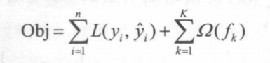
This mathematical formula consists of two parts: the first part is the loss function, which aims to prevent model underfitting (assessing the situation between predicted and actual values), and the second part is the regularization function, which aims to prevent model overfitting (penalizing the parameters of the loss function to prevent model overfitting).

The objective function can be interpreted as the process of learning the “residuals” of predictions from the new model and the previous model. In essence, our optimization goal is to find the optimal f(x) that minimizes the objective function.

Subsequently, we can obtain this minimum objective function through a series of mathematical calculations, completing the entire model construction. However, for our usage, it suffices to understand the conditions for using XGBoost, hyperparameter configuration, and some basic theories.

library(tidyverse)library(mlr3)#https://mlr3book.mlr-org.com/basics.html#taskslibrary(tidymodels)library(ggplot2)library("mlr3verse")library(kknn)library(paradox)#Define the search space for hyperparameterslibrary(mlr3tuning)#For hyperparameter tuninglibrary(ggplot2)

To do a good job, one must first sharpen their tools.

data(Zoo,package = "mlbench")#Import datasetzooTib <- as_tibble(Zoo)#Convert to tibble formatzooXgb <- mutate_at(zooTib,.vars = vars(-type),.funs = as.numeric)

It is important to note that the XGBoost algorithm requires the predictor variables to be numeric, so we need to perform a conversion. However, for categorical variables, blindly converting them may lead to issues, as the qualitative distance between categorical variables is highly valued in machine learning. Therefore, for categorical variables, one can use one-hot encoding, and machine learning can handle multicollinearity issues quite well.

zooTask <- as_task_classif(zooTib, target = "type")#Create tasklrn <- lrn("classif.xgboost")#In fact, XGBoost can also handle regression tasks, but the mlr3 package sets up another function for handling regression tasks.lrn$param_set#Get hyperparameter list

XGBoost has many hyperparameters, but we do not need to master all of them, and tuning hyperparameters does not have a unified standard; it relies more on experience than logic.

#Define hyperparameter search spacesearch_space = ps( eta = p_int(lower = 0, upper = 1), gamma = p_int(lower = 0, upper = 5), max_depth = p_int(lower = 1,upper = 5), nrounds = p_int(lower = 800,upper = 800), subsample = p_dbl(lower = 0.5,upper = 1), eval_metric = p_fct(c("merror","mlogloss")))#eta: learning rate (between 0 and 1), a larger value means slower learning, which can be simply understood as shorter steps. Generally, smaller values are better, while larger values may miss better parameter relationships between data.#max_depth: maximum depth each decision tree can grow.#min_child_weight: minimum purity required before splitting a node (if the node is pure enough, do not split it again).#subsample: proportion of samples randomly drawn (without replacement) for each decision tree; set to 1 to use all samples in the training set (simply put, this makes the samples more representative).#colsample_bytree: essentially prunes each weak learner to prevent overfitting. If a maximum depth is set, this hyperparameter does not need to be adjusted.#nrouds: number of weak learners in the model (generally, do not set it too high, as it may lead to overfitting; experience suggests below 300 is preferable) (however, weak learners and performance generally show a linear trend, meaning we need to select based on our computer's performance. The larger the range, the better).#gamma is the minimum loss reduction required to split a node; if it is 1.0, it means that the loss function must decrease by at least 1.0 at that node to proceed with the split.#eval_metric specifies the evaluation function for the model; for binary classification, it is mainly error, AUC, logloss; for multi-class, it is merror and mlogloss.

The following is based on the concept of nested validation to obtain the most realistic evaluation of the model and to fit the task after obtaining the at variable to achieve the best hyperparameter configuration.

resampling <- rsmp("cv",folds = 10)#Define internal loop resamplingmeasure <- msr("classif.acc")#Define model evaluation metricsevals1000 = trm("evals", n_evals = 1000)#Set tuning stop thresholdtuner = tnr("random_search")#Set tuning algorithmat = AutoTuner$new(lrn, resampling, measure, evals1000 , tuner, search_space)#Package the parameters needed for tuningouter_resampling = rsmp("cv", folds = 5)ptm <- proc.time()rr = resample(zooTask, at, outer_resampling, store_models = TRUE)proc.time() - ptm

Note: Here we set the tuning stop threshold at 1000, meaning that in principle, the model will perform a maximum of 1000 iterations.

rr$aggregate(msr("classif.acc"))#True performance evaluation metric of the model#Since nested validation is not a process for obtaining hyperparameters but to obtain the model's true performance under the best hyperparameter configuration, we only need the evaluation metric of the model.#If we need detailed information from the best hyperparameter modeling, we need to fit the task to trigger at$train(zooTask)#Fit taskat$learner$param_set$values#Get the best hyperparameter configurationat$learner#View XGBoost learner statusat$learner$model#Obtain the XGBoost model with the best hyperparameter configuration, and then perform a series of standard operations, including prediction, etc.#In fact, as a black-box model, it is quite challenging to extract helpful information from XGBoost.

It is important to note that XGBoost, as a black-box model, does not inherently possess good interpretability. Therefore, trying to interpret it like linear regression is not a good idea; we focus more on the model’s performance rather than its interpretability. This brings up the question: when is model interpretability essential?

In summary, we have not only learned about the conventional implementation logic of XGBoost and related coding operations but also understood how to balance machine learning performance and interpretability. Generally speaking, machine learning algorithms, except for pure tree models, do not have particularly excellent interpretability, but they achieve relatively outstanding performance at the expense of interpretability, which is a form of balance.

This article concludes here. For R, XGBoost can be considered a more advanced operation in model building. Everyone can learn and apply it in their project designs, and I believe it will be of great help to you.

I am Chenxi, and see you next time~

Reference Tutorials