
XGBoost (eXtreme Gradient Boosting) is also a member of the Boosting family. To understand its working principle, we first need to briefly introduce the related concepts of AdaBoost and GBDT. AdaBoost focuses on misclassified samples, increasing the weight of misclassified samples each time to train new classifiers. XGBoost is essentially a GBDT, but strives to maximize speed and efficiency, hence the name X (Extreme) GBoost. Interested readers can refer directly to the original article by author Tianqi Chen. Both GBDT and XGBoost belong to the boosting ensemble learning family, with similar boosting strategies focusing on residuals, but differing in how they reduce residuals. GBDT focuses on the residuals of the classifier, aiming to quickly reduce residuals by continuously adding new trees. Each training of the classifier is also aimed at continuously reducing this residual. In fact, if we do not consider some differences in engineering implementation and problem-solving, the biggest difference between XGBoost and GBDT is the definition of the objective function. XGBoost allows the manual definition of the loss function, which can be said to be an engineering implementation of the GBDT algorithm. Roughly speaking, XGBoost is an ensemble machine learning algorithm based on decision trees, using a gradient ascent framework, suitable for classification and regression problems. Its advantages include fast speed, good performance, ability to handle large-scale data, support for multiple languages, and support for custom loss functions.
2 Algorithm Derivation
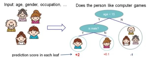
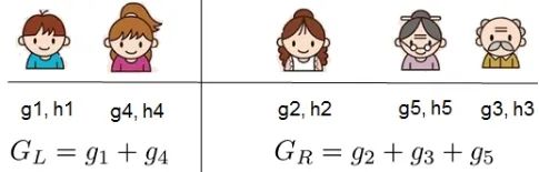
XGBoost is a supervised model, corresponding to the CART tree, where the predicted values of each tree are summed to obtain the final prediction value. The following figure shows a set of CART trees used to determine whether a person likes computer games:
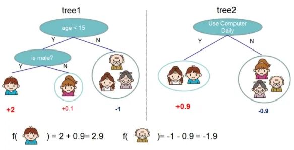
The general idea of using XGBoost to solve the above problem is as follows: first, train the first decision tree, predicting the boy’s desire to play games is 2. This value can be understood as the weight value of the boy’s leaf node. After comparison, it is found to deviate from the label value, leading to the training of the second decision tree, predicting the boy’s desire to play games is 0.9. The two are summed to obtain the final answer of 2.9, further approaching the standard answer. Thus, XGBoost accumulates the weak classification results obtained through training as the final conclusion, which is somewhat similar to GBDT. The two trees above used different attributes as branches, obtaining different values, which are then summed to get the score indicating whether each person likes computer games, ultimately summing to get the total score.
XGBoost uses CART trees rather than ordinary decision trees because, for classification problems, the values corresponding to the leaf nodes of CART trees are actual scores rather than definite categories. This facilitates the implementation of efficient optimization algorithms, which is why XGBoost is known for being both fast and accurate. Mathematically, this model can be accurately represented as follows:
Let k be the number of CART trees, representing the function space of all possible CART trees, and f represents a specific CART tree. Understanding the meaning of f is beneficial for understanding the subsequent algorithm derivation, as it is a decision tree model, where each training sample overall represents the predicted value obtained from the decision tree model for a specific sample, hence can be understood as the output of the leaf node. The overall model consists of k CART trees. Once the model expression is determined, we will focus on explaining the model’s parameters and objective function.
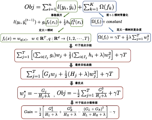
We will first directly present the model’s objective function as follows:
The objective function consists of two parts: the first part is the loss function, which is the number of samples, and the second part is the regularization term, representing the complexity of the tree structure, summed from the regularization terms of k trees.
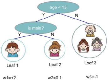
The XGBoost model consists of CART trees, with parameters existing within each CART tree. Determining a CART tree requires defining two parts: the first part is the tree structure (which is a function), responsible for mapping a sample to a specific leaf node. The second part is the score at each leaf node. In GBDT, this score at the leaf node is a parameter that can be trained, but the parameters representing the tree structure are difficult to train, so the algorithm uses additive training to solve this.
2.1 Additive Training
Additive training is essentially a meta-algorithm suitable for all additive models and is a heuristic algorithm. Using additive training, the model objective is not to directly optimize the entire objective function, but rather to optimize the objective function step by step, starting with optimizing the first tree, then optimizing the second tree, until all k trees are optimized. The entire process is shown in the following formula:
At the t step, an optimal CART tree is added, which is the CART tree that minimizes the objective function based on the existing k trees, as follows:
In the above formula, the constant represents the complexity of the previous tree, which can be considered a constant when calculating the tth CART tree. Assuming the loss function used is the squared difference, the above expression can be transformed as follows:
The above expression lacks a constant term at the end, which will be explained later. Note the characteristics of the formula, which contains both linear and quadratic terms, with the coefficient of the linear term being the residual.
2.2 Loss Function
The above only applies to squared difference loss. For other loss functions, similar results may not be obtained. For general loss functions, we need to perform a second-order Taylor expansion, as follows:
Where: g and h.
Then the general loss function can be transformed as:
When optimizing the tth tree, each sample corresponds to the need to calculate the first-order and second-order derivatives, but note that all sums and h have no interconnection, so they can be calculated in parallel, thus accelerating the derivation speed of XGBoost.
Based on the above formula analysis of constants and variables, the constant term is the regularization term of the previous tree, which belongs to constants in the iteration, cumulative error between the previous iteration and the current label, and can also be viewed as a constant term. The remaining three variable terms are the first-order term, second-order term, and regularization term of the tth CART tree (i.e., the value of a certain leaf node). The objective is to minimize the objective function. The constant term can be removed (hence the above expression lacks a constant term), and through simplification, it becomes:
One advantage of XGBoost is that it supports custom loss functions. From the above expression, we can see that the coefficients of the first-order and second-order terms and g can be solved in parallel, and g does not depend on the form of the loss function, as long as the loss function is twice differentiable. Therefore, XGBoost can support custom loss functions, greatly expanding the algorithm’s application scope.
The regularization term of the tth tree (i.e., complexity) is represented by γ, which needs to be determined based on actual needs. To do this, first redefine the structure of the tth CART tree as follows:
First, explain this definition. Suppose a tree has l leaf nodes, the values of these leaf nodes form a l-dimensional vector, which is a mapping function used to map samples into a certain value from 1 to l, i.e., assigning a sample to a specific leaf node, which actually represents the structure of the CART tree. f represents the predicted value of the tree for the sample. According to this definition, XGBoost can use the following regularization term:
The first term is the number of leaf nodes, and the second term is the L2 norm of the weight vector of the leaf nodes. Note: Here appear and , which need to be predefined in XGBoost. When in use, the larger is, the greater the penalty for trees with many leaf nodes, and the objective function will tend to smaller values, making it easier to obtain a simpler structure.
At this point, the optimization objective for the tth tree is already very clear, and we will do the following transformation:
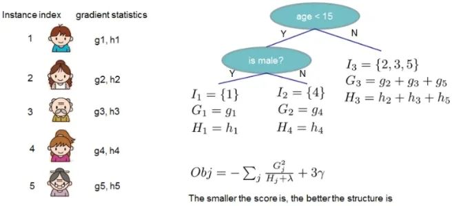
Here I represents a set, where each value in the set represents the index of a training sample, and the entire set consists of the training samples that have been assigned to the jth leaf node of the tth CART tree.
Understanding this, we can see that the transformation above is actually a change in the order of summation, that is, regrouping all training samples according to the leaf nodes. Further simplification can be done as follows:
Where g and h are the sums of the first-order and second-order derivatives of the samples contained in leaf node j, respectively, and are constants;
For a specific structure of the tth CART tree (which can be represented), all sums are determined, and the values of each leaf node in the above expression are independent of each other. The above expression is a simple quadratic form, making it easy to find the optimal value for each leaf node and the value of the objective function at that time. The solution for g is that the objective function can be obtained, and the solution obtained is the weight of each leaf node and the objective function (i.e., the minimum loss brought by the tth tree, which is the regularization loss + training loss) is as follows:
The objective function obj represents the degree of optimization of the tree’s structure. The smaller the value, the better the structure (also known as the structural score), similar to information gain. It is a measure of the quality of the tth CART tree’s structure. Note that this value is only used to measure the tree’s structure, as obj is only related to g and h, and is not related to the values of the leaf nodes, as shown in the following figure:
2.3 Optimal Split Point Algorithm
Although obj can serve as a criterion for evaluating the quality of the tree structure, and the optimal value of the leaf node w has been computed, it seems that the solution for the tth CART tree has been completed. However, the possible structures of the tree are infinite, and it is impractical to test each one individually for their quality and select the best. Therefore, it is still necessary to learn the best tree structure gradually through strategies, which is similar to decomposing the model of the tth tree into multiple single trees for learning, using layer-by-layer node learning. The specific learning process will be understood through examples.
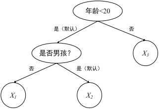
Continuing with the example of determining whether a person likes computer games. The simplest tree structure is a one-node tree, and we can calculate the quality of this single-node tree as obj. Suppose we want to split this single-node tree based on age, we need to calculate:
-
Whether the split by age is effective, i.e., whether it reduces the value of obj;
-
If it is splittable, at which age value should the split be implemented.
To answer these two questions, we can sort the five family members by age, as shown in the following figure:
Scanning from left to right, for each split point a (the vertical line split point in the figure above), calculate g and h, then calculate the split gain score (similar to information gain). The feature with the highest gain score is the optimal split point. XGBoost supports two methods for splitting nodes: greedy algorithm and approximate algorithm.
(1) Greedy Algorithm
a. Start from a tree of depth 0, enumerate all available features for each leaf node;
b. For each feature, sort the training samples belonging to that node in ascending order based on the feature value, and determine the best split point for that feature through linear scanning, recording the split gain;
c. Select the feature with the highest gain as the splitting feature, using the best split point of that feature as the split position, splitting the node into two new leaf nodes, and associating the corresponding sample set for each new node;
d. Return to step b, recursively execute until specific conditions are met.
There are two points that need to be explained: first, the gain calculations for different features can be performed in parallel, which also determines the fast computation speed of XGBoost; second, the feature with the highest gain is selected as the splitting feature.
For each determined split point, the standard for measuring the quality of the split or the split gain calculation process is as follows:
Assuming a feature split is completed at a certain node, the objective function before the split can be written as:
The objective function after the split is:
Then the gain for the objective function after the split is:
Gain actually represents the obj of a single node minus the sum of the obj of the two nodes after the split. When Gain > 0, and the larger this value, the more worthwhile it is to split, indicating that the objective function after the split is smaller than the single-node obj. At the same time, it can be observed that if the left half of Gain is less than the right , then Gain < 0, indicating that the objective function increases after the split, hence the split should not be made. is actually a critical value controlling the level of gain; the larger it is, the stricter the requirements for the decrease in the objective function after the split. By linearly scanning all splits, the optimal split point can be determined. For the two nodes resulting from the split, this splitting process is recursively called, ultimately obtaining a relatively good tree structure.
(2) Approximate Algorithm
The process of building trees using the greedy algorithm in XGBoost traverses all features and their split points, selecting the best one each time. When the data volume is too large, this calculation process can become excessive, so an approximate splitting method can be used, which selects a portion of candidate split points and traverses these points to determine the best split point. Therefore, the selection of candidate split points becomes critical, which will be emphasized below.
Here, a weight quantile sketch algorithm is adopted for dividing candidate points based on the influence of the loss function (Weight Quantile Sketch, WQS). When selecting candidate points, instead of evenly distributing the samples, we aim for uniformity in the distribution of the loss function across the left and right subtrees. Since each sample may contribute differently to reducing the loss function, evenly distributing samples can lead to a significant imbalance in loss distribution between the left and right subtrees, making the constructed tree less applicable, as shown in the figure WQS selects candidate points:
| Sample Index | 1 | 2 | 3 | 4 | 5 | 6 | 7 | 8 | 9 |
|---|---|---|---|---|---|---|---|---|---|
| Feature Value | 1 | 1 | 3 | 4 | 5 | 12 | 45 | 50 | 99 |
| 0.1 | 0.1 | 0.1 | 0.1 | 0.1 | 0.1 | 0.4 | 0.2 | 0.6 | |
| bin1 | bin1 | bin1 | bin1 | bin1 | bin1 | bin2 | bin2 | bin3 |
The second row indicates the values of each sample for a certain feature, and the third row indicates the contribution of each sample to reducing the loss. By following this division, the total contribution of the three categories is 0.6, maintaining relative uniformity. If divided by sample count, the total of the last three samples would be significantly larger than the other six, diminishing the effect of other samples. Hence, the solution is critical, and the following solution process is described.
1) The solution takes the second derivative of the loss function at the sample points, as previously analyzed:
After slight transformation, we obtain:
Each subsequent classifier fits the residual of each sample, and it is evident that the coefficients in front can be viewed as the importance of a sample when calculating the residual, i.e., the contribution of each sample to reducing the loss. By introducing the second derivative into XGBoost, we effectively add weights to the samples based on their contribution when reducing residuals, which can better accelerate fitting and convergence.
2) Binning
The primary task of selecting candidate points is to decide how many bins to divide the sample features into (referred to as binning). Define the dataset, representing the values of the tth feature of n training samples and the second-order gradient values, and define a ranking function.
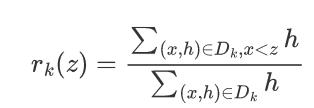
In the above expression, $x
For instance, if $ε$ is set, the division point is at the 1/3 quantile, and the total contribution of samples equals 1.8, then the contribution of each bin should be 1.8*1/3 = 0.6, thus divided into three bins. By first calculating the total contribution and specifying $ε$, reasonable candidate split points can be determined, followed by binning.
During the tree generation process, the selection of each feature’s split points can occur in two scenarios: first is global approximation, proposing all candidate split points during the initial stage of tree construction, then using the same candidate split points for each layer. The candidate split points are not updated, and the number of candidate split points is relatively large; second is local approximation: proposing candidate split points anew for each split, more suitable for deeper trees, with fewer candidate split points required.
After finding the optimal tree structure through the above algorithm, the optimal leaf nodes can be determined according to the tree structure, completing the construction of the tth tree. This algorithm continues to loop until the following conditions are met:
Ⅰ) When the gain introduced by the split is less than the set threshold (gain<0), this split is ignored, similar to the pre-pruning operation in decision trees, where the threshold parameter is the coefficient of the number of leaf nodes in the regularization term ;
Ⅱ) When the tree reaches the maximum depth, the decision tree stops being built, setting a hyperparameter max_depth to avoid the tree growing too deep and learning local samples, thus overfitting;
Ⅲ) When the sum of sample weights is less than the set threshold, tree building stops. After introducing a split, the sample weights for the newly generated left and right leaf nodes are recalculated. If the sample weight of either leaf node falls below a certain threshold, this split is abandoned, similarly preventing overfitting. The calculation method for the sample weight sum of each leaf node is as follows:
Finally, a simple summary of the above derivation is presented in the following figure:
2.4 Several Improvements
In practical engineering applications, some subtle improvements are made to enhance the performance of the XGBoost algorithm, making it increasingly faster and more practical.
(1) Sparse-Aware Algorithm
Sparsity is common in many real-world problems. There are various possible reasons for sparsity:
1) The data contains missing values;
2) Frequent zero entries in statistics;
3) Feature engineering, such as one-hot encoding causing a large amount of sparsity.
During the node construction process, XGBoost only considers the data traversing non-missing values, while adding a default direction for each node. When the feature value corresponding to a sample is missing, the sample can be classified into the default direction.
| Sample | Age | Gender |
|---|---|---|
| – | Male | |
| 15 | – | |
| 25 | Female |
The optimal default direction can be learned from the data. As for how to learn the default value of the branch, it is quite simple: enumerate the samples with missing features into the left and right branches and calculate the gain for each enumeration. The option with the largest gain is the optimal default direction. In simple terms, XGBoost does not assume that missing values must go to the left or right subtree. The first time it assumes that all samples with missing values for a feature go to the right subtree, and the second time it assumes that they all go to the left subtree. The final gains are calculated, and whichever is larger determines the direction.
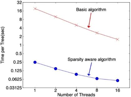
During the tree construction process, enumerating the samples with missing features seems to double the computational load, but actually, the algorithm only considers traversing samples with non-missing features, while samples with missing feature values already have a default direction assigned, thus no further calculation is needed. They can be directly assigned to the left and right nodes, significantly reducing the number of samples that the algorithm needs to traverse. The following figure shows that the sparse-aware algorithm is over 50 times faster than the basic algorithm.
(2) Shrinkage
To prevent excessively large gradients during gradient updates, a shrinkage process is used, meaning that each step taken is small, gradually approaching the result. This method is more effective in avoiding overfitting than taking large steps toward the result. It does not fully trust each residual tree, believing that each tree only learns a small part of the truth. When accumulating, it only adds a small part, compensating for deficiencies by learning several trees. This is clearer when viewed in equation form, where the output of each tree is multiplied by a step size (shrinkage rate), expressed as:

It can be observed that a coefficient less than 1 is added to the last term to reduce its trust level.
(3) Block Structure Design
According to CART tree knowledge, the most time-consuming step in learning is finding the best split point, which requires sorting the feature values each time. XGBoost sorts the data based on features before training, then saves it in a block structure, using a sparse matrix storage format within each block structure during the training process, which can be reused multiple times, significantly reducing computational load.
Each block structure includes one or more sorted features;
Missing feature values will not be sorted;
Each feature stores an index pointing to the sample gradient statistics, facilitating the calculation of first-order and second-order derivative values;
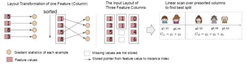
This block structure stores features independently, facilitating parallel computation by computers. When splitting nodes, it is necessary to select the feature with the highest gain as the split feature, allowing the gain calculations for various features to occur simultaneously. This is one of the reasons why XGBoost can achieve distributed or multithreaded computing.
(4) Cache Access Optimization Algorithm
The design of the block structure can reduce the computational load during node splitting, but the design of accessing sample gradient statistics through index can lead to non-contiguous memory space access, resulting in low cache hit rates, thereby affecting algorithm efficiency.
To solve the problem of low cache hit rates, XGBoost proposes a cache access optimization algorithm: allocating a contiguous cache area for each thread to store the required gradient information in the buffer, thus achieving a conversion from non-contiguous to contiguous space, improving algorithm efficiency. Additionally, appropriately adjusting block sizes can also aid in cache optimization.
(5) Out-of-Core Block Computation
When the data volume is too large to load all data into memory, the data that cannot be loaded into memory is temporarily stored on the hard disk, and loaded for computation only when needed. This operation inevitably involves resource wastage and performance bottlenecks due to the speed difference between memory and hard disk. To address this issue, XGBoost assigns a dedicated thread for reading data from the hard disk to enable simultaneous data processing and reading.
Moreover, XGBoost employs two methods to reduce hard disk read and write overhead:
Block compression: compressing blocks by columns and decompressing during reading;
Block splitting: storing each block on different disks, allowing for increased throughput by reading from multiple disks.
3 Algorithm Process
Based on the above analysis, the entire XGBoost algorithm process can be described as follows:
Known: Dataset X and its labels Y, algorithm hyperparameters
To be determined: CART tree classification model
Steps:
-
Define the objective function, including considering the loss of each tree and the complexity of the trees;
-
Use the optimal point splitting algorithm to obtain feature split points, calculating tree loss while calculating tree complexity;
-
Output the final result, compare it with the labels, and update parameters using the residual;
-
Terminate the algorithm based on stopping iteration conditions and output the model.
Note: The splitting operation in XGBoost is different from that of ordinary decision trees. Ordinary decision trees do not consider the tree’s complexity during splitting, relying instead on subsequent pruning operations for control. XGBoost already considers the tree’s complexity during splitting, which is the parameter . Thus, it does not require separate pruning operations. It is evident that XGBoost employs the same idea as CART regression trees, utilizing a greedy algorithm to traverse all features and their split points. The difference lies in the objective function used. The specific approach is that the post-split objective function value must exceed the gain of the single leaf node’s objective function, and to limit the tree from growing too deep, a threshold is added. Only when the gain exceeds this threshold will a split occur, continuing to split, forming one tree after another, each time further splitting/building based on the previous prediction.
4 Case Analysis
Suppose we want to predict students’ exam scores, given several student attributes (such as talent, daily study time, family environment, etc.):
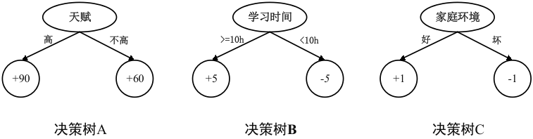
Through decision tree A, those with high talent score +90, while those without score +60;
Through decision tree B, those studying more than 10 hours a day score +5, while those studying less score -5;
Through decision tree C, those from good family environments score +1, while those from poor environments score -1.
Following this process, more decision trees might be generated to infer scores based on student attributes. XGBoost is an algorithm that continuously generates new decision trees A, B, C, D… The final decision tree algorithm is the sum of trees A+B+C+D+…
For this problem, let’s look at the detailed tree-building process:
Initially, there are three students, with attributes and labels as follows: initializing the predicted exam scores of the three samples to 0.
| Sample | Talent | Study Time | Family Environment | Score |
|---|---|---|---|---|
| X1 | High | 16h | Good | 100 |
| X2 | Low | 16h | Good | 70 |
| X3 | High | 6h | Good | 86 |
Assuming a decision tree A has already been established based on the talent attribute (note that this premise is that the split gain has determined the split point based on talent).

With the first tree, the prediction results are:
| Sample | Talent | Study Time | Family Environment | Score | Decision Tree A Prediction | Difference with Label |
|---|---|---|---|---|---|---|
| X1 | High | 16h | Good | 100 | 90 | 10 |
| X2 | Low | 16h | Good | 70 | 60 | 10 |
| X3 | High | 6h | Good | 86 | 90 | -4 |
When establishing the second tree, only the residuals need to be considered, meaning the samples actually become as follows:
| Sample | Talent | Study Time | Family Environment | Difference with Label |
|---|---|---|---|---|
| X1 | High | 16h | Good | 10 |
| X2 | Low | 16h | Good | 10 |
| X3 | High | 6h | Good | -4 |
By minimizing the residuals, a decision tree based on study time is learned, resulting in predictions of 90+5, 60+5, and 90-5. The process continues through the real values and the current predictions (100-95=5), (70-65), and (86-85) to build the next decision tree. This continues until the iteration limit is reached or the residuals stop decreasing, resulting in a strong classifier consisting of multiple (iteration count) decision trees. This is the macro process of XGBoost.
5 Algorithm Summary
The impact of XGBoost has been widely recognized in store sales forecasting; high-energy physics event classification; online text classification; customer behavior prediction; sports detection; advertisement click-through rate prediction; malware classification; product classification; risk prediction; and large-scale online course dropout rate prediction. Now, XGBoost has developed into an optimized distributed gradient boosting library aimed at achieving efficiency, flexibility, and portability.
To summarize the advantages of this algorithm:
Higher accuracy: GBDT only uses first-order Taylor expansion, while XGBoost performs second-order Taylor expansion on the loss function. The introduction of the second derivative in XGBoost serves to increase accuracy and allows for custom loss functions, as second-order Taylor expansion can approximate a large number of loss functions;
Greater flexibility: GBDT uses CART as the base classifier, while XGBoost supports not only CART but also linear classifiers (using linear classifiers in XGBoost is equivalent to logistic regression with L1 and L2 regularization terms for classification problems or linear regression for regression problems). Additionally, the XGBoost tool supports custom loss functions, requiring only that the function supports first-order and second-order derivatives;
Regularization: XGBoost incorporates regularization terms into the objective function to control model complexity. The regularization term includes the number of leaf nodes in the tree and the L2 norm of the leaf node weights. The regularization term reduces the model’s variance, making the learned model simpler, which helps prevent overfitting;
Shrinkage: equivalent to the learning rate. After each iteration, XGBoost multiplies the weights of the leaf nodes by this coefficient, mainly to weaken the influence of each tree, allowing more learning space for subsequent trees;
Column sampling: XGBoost adopts a method similar to random forests, supporting column sampling, which not only reduces overfitting but also decreases computation;
Handling missing values: The sparse-aware algorithm employed by XGBoost greatly accelerates node splitting speed;
Parallelizable operations: The block structure supports parallel computation effectively.
Disadvantages:
Although pre-sorting and approximate algorithms can reduce the computational load of finding the best split points, the data set still needs to be traversed during node splitting;
The space complexity of the pre-sorting process is too high, requiring storage of both feature values and the corresponding gradient statistics index of the samples, effectively consuming double the memory.