1. Data Processing
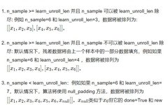
The mini-batch data used for training RNNs differs from the usual data. This data should typically be arranged in a time series. For DI-engine, this processing is done during the collector phase. Users need to specify learn_unroll_len in the configuration file to ensure that the length of the sequence data matches the algorithm. In most cases, learn_unroll_len should equal the historical length of the RNN (a.k.a. time series length), but this is not always the case. For example, in R2D2, we use burn-in operations, where the sequence length equals learn_unroll_len + burnin_step. This will be explained in detail in the next section.
What is Data Processing?
Data processing refers to the process of preparing time series data for training recurrent neural networks (RNNs). This process includes organizing the collected data into appropriately formatted mini-batches that will be used for training the network. This step usually occurs in the collector phase of DI-engine, where data collection and preprocessing take place. Users need to specify learn_unroll_len in the configuration file to ensure that the length of the sequence data matches the algorithm. In most cases, learn_unroll_len should equal the historical length of the RNN (a.k.a. time series length), but this is not always the case. For example, in R2D2, we use burn-in operations, where the sequence length equals learn_unroll_len + burnin_step. For instance, if you set learn_unroll_len = 10 and burnin_step = 5, then the actual input sequence length received by the RNN will be 15: the first 5 steps are burn-in (to warm up the hidden state), followed by 10 steps as part of the learning. This setup helps the RNN have a more accurate hidden state as a starting point when computing gradients and performing weight updates.
Explanation of Some Terms
Mini-batches: In machine learning, especially when training neural networks, data is generally divided into small batches for processing, referred to as “mini-batches”. A mini-batch contains a set of samples used to perform a single iteration of forward and backward propagation to update the network’s weights. Using mini-batches instead of a single sample or the entire dataset (the latter referred to as “batch” or “full-batch”) can balance computational efficiency and memory constraints, helping to improve learning stability and convergence speed.
Collector Phase: In DI-engine, the collector phase refers to the process where the environment interacts with the agent and collects experience data. During this phase, the agent performs actions based on its current policy, and the environment returns new states, rewards, and other possible information, such as whether the termination state has been reached. The collected data (often referred to as experiences or transitions) is then used to train the agent’s model, such as updating the policy or value function.
Why Data Processing is Necessary:
1. Maintain Temporal Dependency: The core advantage of RNNs is their ability to handle data with temporal dependencies, such as language, video frames, stock prices, etc. Proper data processing ensures that these temporal dependencies are preserved in the training data, allowing the model to learn the sequential features within the data.
2. Improve Learning Efficiency: By dividing the data into batches that match the expected sequence length of the model, the efficiency of model learning can be improved. This ensures that the network receives sufficient contextual information during each update.
3. Adapt to Algorithm Requirements: Different RNN algorithms may require different forms of input data. For example, standard RNNs only need past information, while some variants like LSTM or GRU may handle longer sequences. Specific algorithms, like R2D2, may also require additional steps (like burn-in) to better initialize the network state.
4. Handle Irregular Lengths: In real-world datasets, sequence lengths are often irregular. Data processing ensures that each mini-batch has a uniform sequence length, typically achieved by truncating overly long sequences or padding shorter ones.
5. Optimize Memory and Computational Resources: By organizing data into batches with fixed time steps, GPU and other computational resources can be utilized more efficiently since these resources are generally more efficient at processing fixed-size data.
6. Stabilize the Learning Process: Especially in reinforcement learning, using techniques like n-step returns or experience replay can help the model learn from environmental feedback and reduce variance, thereby stabilizing the learning process.
How to Process Data
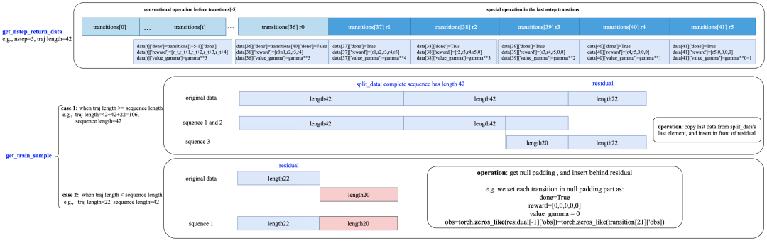
Taking the R2D2 algorithm as an example, in R2D2, the method _get_train_sample retrieves the time-ordered data by calling the functions get_nstep_return_data and get_train_sample.
def _get_train_sample(self, data: list) -> Union[None, List[Any]]: data = get_nstep_return_data(data, self._nstep, gamma=self._gamma) return get_train_sample(data, self._sequence_len)The code segment def _get_train_sample(self, data: list) is a method that extracts samples used for training the RNN from the collected data. This method processes the data in two steps:
N-step return calculation (get_nstep_return_data): This function takes the raw experience data and calculates what is known as the N-step return value. The N-step return is a concept used in reinforcement learning for Temporal Difference (TD) learning, which considers the cumulative reward over the next N steps starting from the current state. Calculating this value requires the use of a discount factor gamma. The purpose of this step is to allow the agent to learn how to predict future rewards based on its current actions, which is an important part of value function estimation in reinforcement learning.
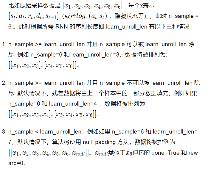
Training sample acquisition (get_train_sample): After obtaining the N-step return values, this function further processes the data to generate training samples. Specifically, it selects a data sequence based on self._sequence_len (i.e., the time series length or the historical length of the RNN). This means that each training sample will be a data sequence of length self._sequence_len, which is necessary for training the RNN because the RNN needs a certain length of history to maintain its internal state (or memory).
For the workflow of these two data processing functions, see the diagram below:
2. Initializing the Hidden State
RNNs are used to process information with temporal dependencies. The hidden state of the RNN is part of its memory, capable of capturing information from the previous time step. This information is crucial for predicting the next action or state. In this context, initializing the hidden state of the RNN is an important step, ensuring that the RNN has the correct starting state when beginning to process a new batch of data.
The policy’s _learn_model needs to initialize the RNN. These hidden states come from _collect_model saved prev_state. Users need to add these states to the _learn_model input data dictionary via the _process_transition function.
def _process_transition(self, obs: Any, model_output: dict, timestep: namedtuple) -> dict: transition = { 'obs': obs, 'action': model_output['action'], 'prev_state': model_output['prev_state'], # add ``prev_state`` key here 'reward': timestep.reward, 'done': timestep.done, } return transitionThis function processes the observations, model outputs, and timestep information collected from the environment for each time step, organizing them into a dictionary called transition, which includes the following key-value pairs:
‘obs’: Current observation.
‘action’: Action from the model output.
‘prev_state’: The previous hidden state from the model output, which is the internal state of the RNN before the current step.
‘reward’: Reward for the current time step.
‘done’: Indicates whether the current time step is the end of the sequence.
Storing prev_state
In the transition dictionary, the ‘prev_state’ key stores the previous hidden state from the model output, which will be used to initialize the hidden state of the RNN in _learn_model.
Then, in the _learn_model forward function, its reset function (corresponding to the reset function inside HiddenStateWrapper) is called to initialize the RNN’s prev_state.
def _forward_learn(self, data: dict) -> Dict[str, Any]: # forward data = self._data_preprocess_learn(data) self._learn_model.train() self._learn_model.reset(data_id=None, state=data['prev_state'][0])This is the forward propagation function of the learning model of the policy. In this function, the hidden state of the RNN is initialized by calling the model’s reset function. This is done at the beginning of each training batch to ensure that the RNN starts learning from the correct state.
The reset function is part of the HiddenStateWrapper class, responsible for resetting the internal state of the RNN.
Burn-in (in R2D2)
The concept of burn-in comes from the R2D2 (Recurrent Experience Replay In Distributed Reinforcement Learning) paper. In the R2D2 algorithm, since LSTMs need to handle time series data, they require a reasonable initial hidden state. The burn-in period allows the LSTM to “warm up” by processing some initial sequence data, enabling it to build some meaningful internal state before officially starting to learn. The paper notes that when using LSTMs, the most basic approach is:
1. Split the complete episode trajectory into many sequence samples. At the initial moment of each sequence sample, use a tensor of all zeros as the initialization hidden state for the RNN.
2. Use the complete episode trajectory for RNN training.
For the first method, since the hidden state at the initial moment of each sequence sample should contain information from prior moments, simply using a tensor of all zeros introduces significant bias. For the second method, the length of a complete episode often varies across different environments, making it difficult to use directly for RNN training.
Burn-in gives the RNN network a burn-in period, i.e., using the initial part of the replay sequence to generate a starting hidden state, and then only updating the RNN network on the latter part of the replay sequence.
In DI-engine, R2D2 uses n-step TD error, that is, self._nstep is the number of n. The sequence length = burnin_step + learn_unroll_len. Therefore, in the configuration file, learn_unroll_len should be set to sequence length – burnin_step.
In this setup, the original unfolded observation sequence is split into burnin_nstep_obs, main_obs, and target_obs. burnin_nstep_obs is used to compute the initial hidden state of the RNN, which will later be used to calculate q_value, target_q_value, and target_q_action. main_obs is used to calculate q_value. In the code below, [bs:-self._nstep] indicates using data from time step bs to sequence length – self._nstep. target_obs is used to calculate target_q_value.
This data processing can be implemented with the following code:
data['action'] = data['action'][bs:-self._nstep]data['reward'] = data['reward'][bs:-self._nstep]data['burnin_nstep_obs'] = data['obs'][:bs + self._nstep]data['main_obs'] = data['obs'][bs:-self._nstep]data['target_obs'] = data['obs'][bs + self._nstep:]Specific to the code analysis:
data[‘action’] and data[‘reward’] slice [bs:-self._nstep] indicates taking from the bs time step of the sequence to the last self._nstep time step. bs represents the burn-in steps, ensuring that the actions and rewards correspond to the time steps of the predicted Q-value when calculating TD errors.
data[‘burnin_nstep_obs’] stores the observation sequence used for calculating the initial hidden state of the RNN. The [:bs + self._nstep] slice means taking from the start of the sequence up to the bs + self._nstep time step. This portion of data will not be used for gradient updates, only for generating the initial state of the RNN.
data[‘main_obs’] represents the main observation sequence used for actual Q-value calculations. It is obtained through the slice [bs:-self._nstep], ensuring that the main observation sequence excludes the portion used for burn-in and the last few steps used for calculating the target Q-value (as n-step TD errors are needed).
data[‘target_obs’] stores the observation sequence used for calculating the target Q-value. The slice [bs + self._nstep:] means starting from the burn-in period plus n steps until the end of the sequence.
When using burn-in techniques in the R2D2 algorithm, it is necessary to update and save the RNN’s hidden state at each time step so that the correct state can be used to initialize the RNN during the learning phase. Since the RNN’s hidden state is based on time series, it is crucial to adopt appropriate methods to handle this.
Collecting Model (self._collect_model)
When calling the forward method of self._collect_model for data collection, inference=True is typically set. In this mode, only a single time step of data is processed each time, allowing the current hidden state (prev_state) of the RNN to be obtained at each time step.
Learning Model (self._learn_model)
During the learning phase, when calling the forward method of self._learn_model, inference=False is set. In non-inference mode, a series of data is passed in, and the output’s prev_state field only represents the hidden state of the last time step in the sequence.
Saving Hidden State at Specific Time Steps
To save the hidden state at specific time steps other than the last one, the saved_hidden_state_timesteps parameter can be specified. This parameter is a list indicating the time steps at which the hidden state needs to be saved.
Application in R2D2
In the implementation of R2D2, by specifying saved_hidden_state_timesteps=[self._burnin_step, self._burnin_step + self._nstep], specific time steps’ hidden states can be saved in burnin_output and burnin_output_target after calling the network’s forward method. These saved hidden states will be used in subsequent calculations, such as calculating Q-values (q_value), target Q-values (target_q_value), and target actions (target_q_action).
Example Code
def _forward_learn(self, data: dict) -> Dict[str, Any]: # forward data = self._data_preprocess_learn(data) self._learn_model.train() self._target_model.train() # use the hidden state in timestep=0 self._learn_model.reset(data_id=None, state=data['prev_state'][0]) self._target_model.reset(data_id=None, state=data['prev_state'][0]) if len(data['burnin_nstep_obs']) != 0: with torch.no_grad(): inputs = {'obs': data['burnin_nstep_obs'], 'enable_fast_timestep': True} burnin_output = self._learn_model.forward( inputs, saved_hidden_state_timesteps=[self._burnin_step, self._burnin_step + self._nstep] ) burnin_output_target = self._target_model.forward( inputs, saved_hidden_state_timesteps=[self._burnin_step, self._burnin_step + self._nstep] ) self._learn_model.reset(data_id=None, state=burnin_output['saved_hidden_state'][0]) inputs = {'obs': data['main_obs'], 'enable_fast_timestep': True} q_value = self._learn_model.forward(inputs)['logit'] self._learn_model.reset(data_id=None, state=burnin_output['saved_hidden_state'][1]) self._target_model.reset(data_id=None, state=burnin_output_target['saved_hidden_state'][1]) next_inputs = {'obs': data['target_obs'], 'enable_fast_timestep': True} with torch.no_grad(): target_q_value = self._target_model.forward(next_inputs)['logit'] # argmax_action double_dqn target_q_action = self._learn_model.forward(next_inputs)['action']This code snippet is an implementation example of the learning process in the R2D2 algorithm, demonstrating how to combine burn-in techniques and RNNs in a reinforcement learning model. The code is mainly divided into several parts:
1. Data Preprocessing: self._data_preprocess_learn(data) may perform some normalization or other preprocessing steps on the input data.
2. Setting Models to Training Mode: self._learn_model.train() and self._target_model.train() set both models to training mode, which enables gradient computation in PyTorch.
3. Resetting Model State: Using self._learn_model.reset() and self._target_model.reset() to initialize both models’ hidden states to data[‘prev_state’][0], which is the hidden state of the first time step in the sequence.
4. Executing the Burn-in Process: If data[‘burnin_nstep_obs’] is not empty, indicating the presence of a burn-in sequence, the burn-in process is executed. Within the torch.no_grad() context, this means that gradients will not be computed during this process. burnin_output and burnin_output_target save the outputs of the learning model and target model after the burn-in steps, including the saved hidden states.
5. Calculating Q-values: The code then sets the hidden state of the learning model to the last state from the burn-in phase using self._learn_model.reset(), preparing to calculate the Q-values for the main observation sequence data[‘main_obs’]. q_value is the Q-value calculated based on the main observation sequence.
6. Calculating Target Q-values and Target Actions: Next, the hidden states of the learning model and target model are set to the second state calculated during the burn-in phase using self._learn_model.reset() and self._target_model.reset(). This state is used to calculate the target Q-value (target_q_value) and target action (target_q_action) for the next observation sequence (data[‘target_obs’]), which are used to update the Q-network’s parameters.
The key aspect of this code is that it uses a burn-in sequence to generate the initial hidden state of the RNN, which is then used to calculate the Q-values for subsequent sequences. This approach helps mitigate the bias introduced by initializing the hidden state to zero. Additionally, the code demonstrates how to handle hidden states at different time steps, which is crucial for RNNs when processing time series data. In reinforcement learning, this handling method helps improve the stability and performance of the algorithm.