
Date:August 28, 2019
Word Count:2400words, 11images
Estimated Reading Time:7minutes
Source:Machine Heart
This article is selected from Medium, mainly introducing convolutional neural networks in neural networks, suitable for beginners to read.
Overview
Deep learning and artificial intelligence were buzzwords in 2016; in 2017, these two terms became even more popular, but also more confusing. We will delve into the core of deep learning, which is neural networks. Most variants of neural networks are difficult to understand, and their underlying structural components make them theoretically and graphically similar.
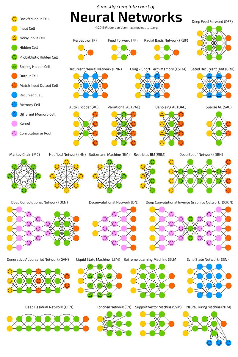
The diagram below shows the most popular variants of neural networks, which can be referenced in this blog (http://www.asimovinstitute.org/neural-network-zoo/).
This article introduces convolutional neural networks (CNNs). Before we start, let’s first understand the perceptron. A neural network is a collection of units called perceptrons, which are binary linear classifiers.
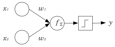
As shown in the figure above, the inputs x1 and x2 are multiplied by their respective weights w1 and w2 and summed, so the function f=x1*w1+x2*w2+b (bias term, which can be optionally added). The function f can be any operation, but for perceptrons, it is usually a summation. The function f is then evaluated by an activation function that can achieve the desired classification. The sigmoid function is the most common activation function used for binary classification. If you want to learn more about perceptrons, I recommend reading this article (https://appliedgo.net/perceptron/).
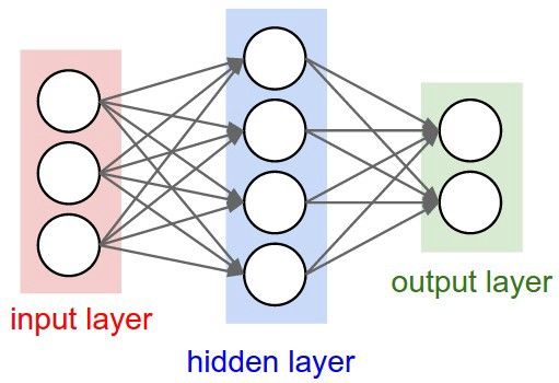
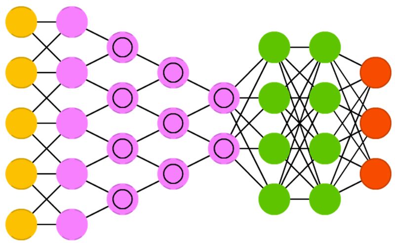
If we stack multiple inputs together and use function f to connect them with multiple stacked units in another layer, we form multiple fully connected perceptrons, and the outputs of these units (hidden layers) become the inputs to the final unit, which then obtains the final classification through function f and the activation function. As shown in the figure below, this is the simplest neural network.
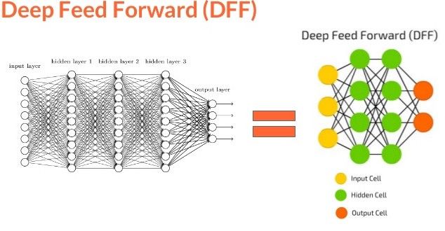
Neural networks have a unique capability known as the Universal Approximation function, so the topology and structural variants of neural networks are diverse. This itself is a large topic, and Michael Nielsen describes it in detail in his article (http://neuralnetworksanddeeplearning.com/chap4.html). After reading this, we can believe that neural networks can simulate any function, no matter how complex it is. The aforementioned neural networks are also called feedforward neural networks (FFNN), as the flow of information is unidirectional and acyclic. Now that we understand the basic knowledge of perceptrons and feedforward neural networks, we can imagine that hundreds of inputs connected to several such hidden layers will form a complex neural network, often referred to as a deep neural network or deep feedforward neural network.
So what is the difference between deep neural networks and convolutional neural networks? Let’s explore.
CNNs have gained popularity due to their application in competitions like ImageNet and have recently been applied in natural language processing and speech recognition. The key point to remember is that other variants, such as RNNs, LSTMs, and GRUs, are based on structures similar to CNNs, although there are some architectural differences.
CNNs consist of three different layers: the convolutional layer, the pooling layer, and the dense or fully connected layer. The neural networks we discussed earlier are typical fully connected layer neural networks. To learn more about convolutional and pooling layers, you can read Andrej Karpathy’s explanation (https://cs231n.github.io/convolutional-networks/). Now let’s continue our discussion about layers, and next, we will look at the convolutional layer.
(In the following content, we will use image classification as an example to understand convolutional neural networks, and later shift to natural language processing and video tasks.)
Convolutional Layer: Suppose an image has 5*5 pixels, where 1 represents white and 0 represents black; this image is viewed as a 5*5 monochrome image. Now, we use a 3*3 matrix composed of random 0s and 1s to perform multiplication with sub-regions of the image, moving one pixel at a time in each iteration, resulting in a new 3*3 matrix. The animated image below illustrates this process.
The above 3*3 matrix is called a filter, and its task is to extract features from the image. It uses an optimization algorithm to determine the specific 0s and 1s in the 3*3 matrix. In the convolutional layer of the neural network, we use several such filters to extract multiple features. Each individual step of the 3*3 matrix is called a stride.
The diagram below shows the detailed process of generating two convolution outputs from a three-channel (RGB) image using two three-channel filters.
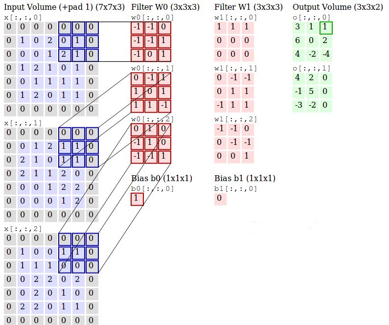
Filters w0 and w1 are convolutions, and the outputs are the extracted features; the layer containing these filters is called the convolutional layer.
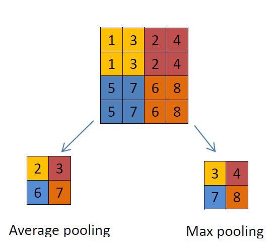
Pooling Layer: This layer primarily uses different functions to reduce the dimensionality of the input. Typically, the max pooling layer appears after the convolutional layer. The pooling layer processes the image in the same way as the convolutional layer but reduces the dimensionality of the image itself. Below are examples of using max pooling and average pooling.
Fully Connected Layer: This layer is the fully connected layer that lies between the previous layer and the activation function. It is similar to the simple neural network we discussed earlier.
Note: The results of convolutional neural networks also use regularization layers, but this article will discuss them separately. Additionally, the pooling layer loses information, so it is not the preferred choice. The usual practice is to use a larger stride in the convolution layer.
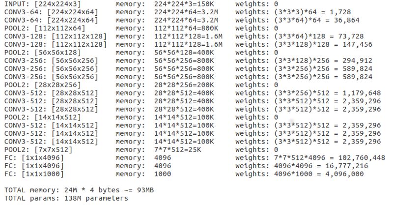
VGGNet, the runner-up of ILSVRC 2014, is a popular convolutional neural network that uses 16 layers to help us understand the importance of depth in CNNs. AlexNet, the champion of ILSVRC 2012, only has 8 layers. There is a model VGG-16 in Keras that can be used directly.
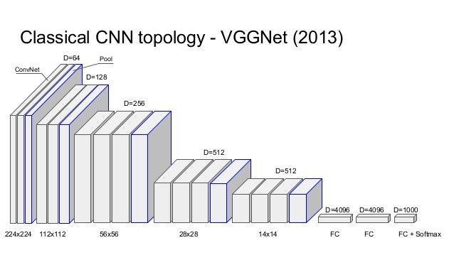
After loading this model in Keras, we can observe the “output shape” of each layer to understand the tensor dimensions and observe the “Param#” to understand how to calculate parameters to obtain convolution features. “Param#” refers to all weight updates each time convolution features are obtained.
Now that we are familiar with the structure of convolutional neural networks and understand how each layer operates, we can further comprehend how it is applied in natural language processing and video processing. You can learn about all the CNN models that have won the ImageNet competition since 2012 at this link (https://adeshpande3.github.io/The-9-Deep-Learning-Papers-You-Need-To-Know-About.html).