
Source:DeepHuhb IMBA
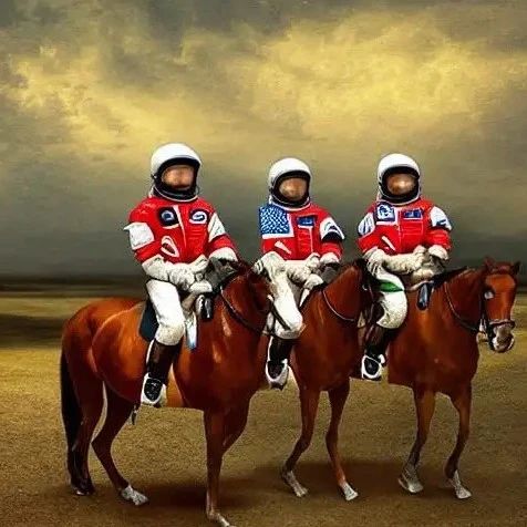
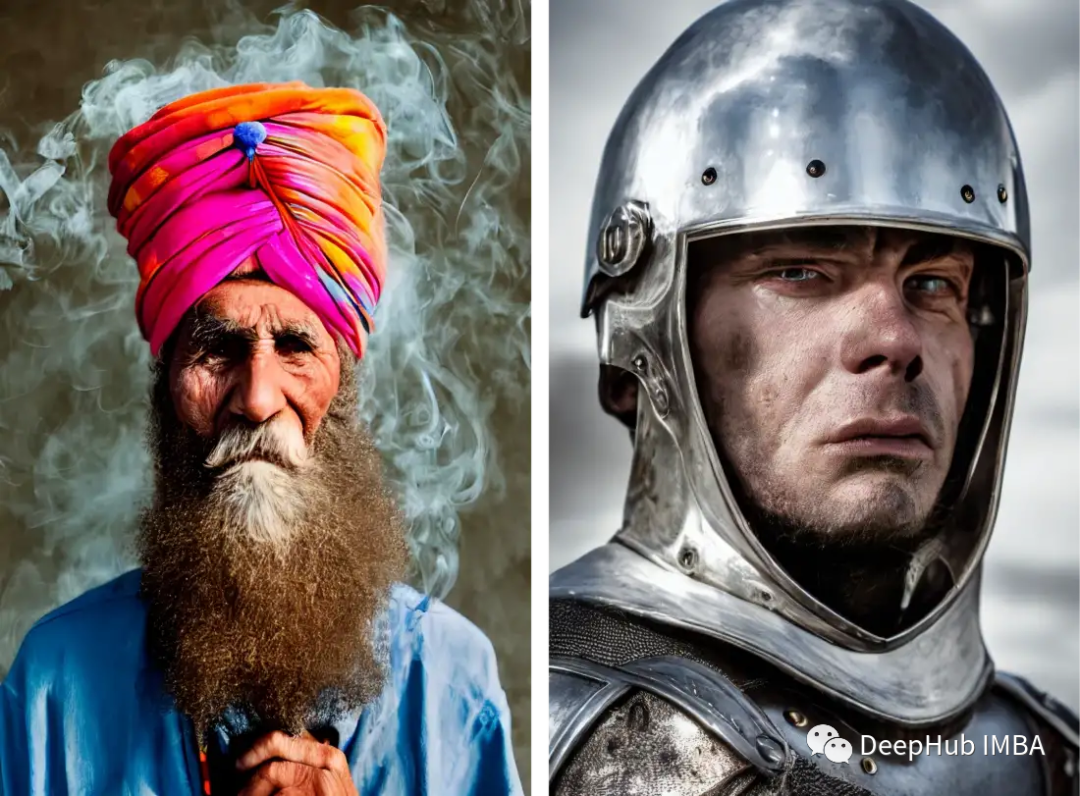
Stable Diffusion is a latent diffusion model for text-to-image generation, created by researchers and engineers from CompVis, Stability AI, and LAION. It is trained on 512×512 images from a subset of the LAION-5B database. Using this model, any image, including faces, can be generated. Since there are open-source pre-trained models available, we can also run it on our own machines, as shown in the figure below.
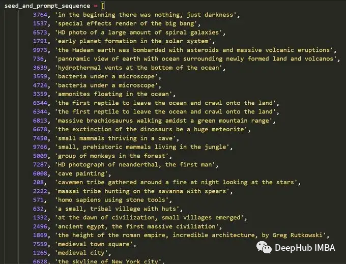
If you are clever and creative enough, you can create a series of images and then form a video. For example, Xander Steenbrugge used it along with the input prompt shown in the above image to create the stunning “Through Time”.
Below is the inspiration and text he used to create this creative artwork:
This article first introduces what Stable Diffusion is and discusses its main components. Then we will create images using the model in three different ways, ranging from simpler to more complex.
Stable Diffusion
Stable Diffusion is a machine learning model that is trained to progressively denoise random Gaussian noise to obtain samples of interest, such as generating images.
The main disadvantage of diffusion models is that the denoising process is very expensive in terms of time and memory consumption. This can slow down the process and consume a lot of memory. The main reason is that they operate in pixel space, especially when generating high-resolution images.
Latent diffusion reduces memory and computational costs by applying the diffusion process in a lower-dimensional latent space instead of using the actual pixel space. Therefore, Stable Diffusion introduces the method of Latent diffusion to address this costly computational issue.
1. Main Components of Latent Diffusion
Latent diffusion has three main components:
Autoencoder (VAE)
The autoencoder (VAE) consists of two main parts: the encoder and the decoder. The encoder transforms images into a low-dimensional latent representation, which serves as input for the next component, U_Net. The decoder does the reverse, converting the latent representation back into images.
During the training process of Latent diffusion, the encoder is used to obtain the latent representation of the input image during the forward diffusion process. During inference, the VAE decoder converts the latent signal back into images.
U-Net
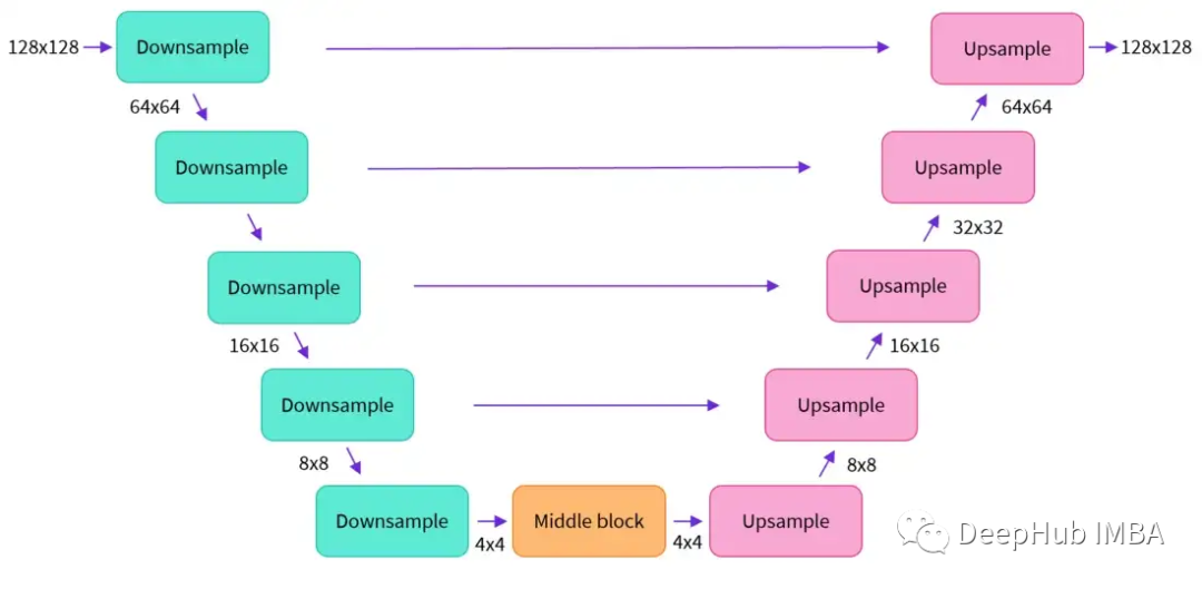
U-Net also includes both encoder and decoder parts, both of which consist of ResNet blocks. The encoder compresses the image representation into a low-resolution image, while the decoder decodes the low-resolution image back into a high-resolution image.
To prevent U-Net from losing important information during downsampling, shortcut connections are typically added between the downsampled ResNet of the encoder and the upsampled ResNet of the decoder.
The U-Net in Stable Diffusion adds cross-attention layers to modulate the output of the text embeddings. Cross-attention layers are added between the encoder and decoder ResNet blocks of U-Net.
Text-Encoder
The text encoder converts the input text prompts into an embedding space that U-Net can understand. It is a simple transformer-based encoder that maps token sequences to latent text embedding sequences. From here, it can be seen that using good text prompts leads to better expected outputs.
Why Latent Diffusion is Fast and Efficient
Latent Diffusion is fast and efficient because its U-Net operates in a low-dimensional space. Compared to pixel space diffusion, this reduces memory and computational complexity. For example, an image of size (3,512,512) in latent space becomes (4,64,64), reducing memory by 64 times.
Inference Process of Stable Diffusion
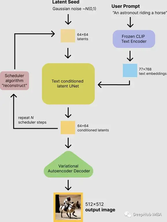
First, the model takes a random seed from the latent space and the text prompt as inputs simultaneously. Then, a random latent image representation of size 64×64 is generated using the seed in the latent space, while the input text prompt is converted into a text embedding of size 77×768 through the CLIP text encoder.
Next, U-Net iteratively denoises the random latent image representation while conditioning on the text embedding. The output of U-Net is the noise residual, which is used to calculate the denoised latent image representation through the scheduler algorithm. The scheduler algorithm computes the predicted denoised image representation based on the previous noise representation and the predicted noise residual.
Many different scheduler algorithms can be used for this computation, each with its advantages and disadvantages. For Stable Diffusion, it is recommended to use one of the following:
-
PNDM scheduler (default)
-
DDIM scheduler
-
K-LMS scheduler
The denoising process is repeated about 50 times to gradually retrieve better latent image representations. Once completed, the latent image representation is decoded by the decoder part of the variational autoencoder.
Using Hugging Face’s API
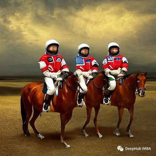
Hugging Face provides a very simple API to use our model for generating images. In the figure below, I used “astronaut riding a horse” as input to get the output image:
The model they provide also includes some advanced options to change the quality of the generated images, as shown in the figure below:

The four options here are described as follows:
images: This option controls the maximum number of generated images, which can be up to 4.
Steps: This option selects the number of steps for the desired diffusion process. The more steps, the better the quality of the generated image. If high quality is desired, the maximum available number of steps, which is 50, can be selected. If faster results are desired, consider reducing the number of steps.
Guidance Scale: The Guidance Scale is a trade-off between the tightness of the generated images to the input prompt and the diversity of the input. Its typical value is around 7.5. The higher the scale, the better the quality of the image, but the less diverse the output will be.
Seed: The random seed controls the diversity of the generated samples.
Using the Diffuser Package
The second method of use is to utilize Hugging Face’s Diffusers library, which includes most of the currently available stable diffusion models that we can run directly on Google Colab.
The first step is to open Google Colab and check if it is connected to a GPU, which can be viewed in the resource button, as shown in the figure below:

Another option is to select “Change runtime type” from the Runtime menu and ensure the hardware accelerator is selected as GPU:

Once we ensure we are using a GPU runtime, we can use the code below to check which GPU we got:
!nvidia-smi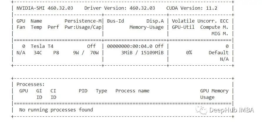
Unfortunately, we only got a T4 allocated, if you can allocate a P100, then your inference speed will be faster.
Next, we install some required packages: diffusers, scipy, ftfy, and transformers:
!pip install diffusers==0.4.0 !pip install transformers scipy ftfy !pip install "ipywidgets>=7,<8"Additionally, it is necessary to agree to the model agreement and accept the model license by checking the checkbox. Register on “Hugging Face” and get an access token, etc.
Moreover, for Google Colab, it has disabled external widgets, so it needs to be enabled. Run the following code to use “notebook_login”
from google.colab import output output.enable_custom_widget_manager()You can now log in to Hugging Face using the access token obtained from your account:
from huggingface_hub import notebook_login notebook_login()Load the StableDiffusionPipeline from the diffusers library.
StableDiffusionPipeline is an end-to-end inference pipeline used to generate images from text.
We will load the pre-trained model weights. The model id will be CompVis/stable-diffusion-v1-4, and we will also use a specific type of revision for the torch_dtype function. Setting revision = “fp16” loads the weights from the half-precision branch and sets torch_dtype = “torch.float16” to tell the model to use fp16 weights.
This setup can reduce memory usage and run faster.
import torch from diffusers import StableDiffusionPipeline # make sure you're logged in with `huggingface-cli login` pipe = StableDiffusionPipeline.from_pretrained("CompVis/stable-diffusion-v1-4", revision="fp16", torch_dtype=torch.float16) Next, set up the GPU:
pipe = pipe.to("cuda")Now we can generate images. We will write a prompt text and feed it to the pipeline and print the output. The input prompt here is “an astronaut riding a horse”; let’s see the output:
prompt = "a photograph of an astronaut riding a horse" image = pipe(prompt).images[0] # image here is in [PIL format](https://pillow.readthedocs.io/en/stable/) # Now to display an image you can do either save it such as: image.save(f"astronaut_rides_horse.png")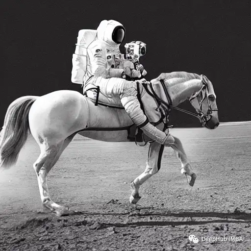
Every time you run the code above, you will get a different image. To get the same result each time, you can pass a random seed as shown in the code below:
import torch generator = torch.Generator("cuda").manual_seed(1024) image = pipe(prompt, generator=generator).images[0] imageYou can also change the number of steps using the num_inference_steps parameter. Generally, the more inference steps, the higher the quality of the generated image, but it takes more time to generate results. If you want faster results, you can use fewer steps.
The cell below uses the same seed as before but with fewer steps. Note some details, such as the horse’s head or helmet, are defined more vaguely than in the previous image:
import torch generator = torch.Generator("cuda").manual_seed(1024) image = pipe(prompt, num_inference_steps=15, generator=generator).images[0] image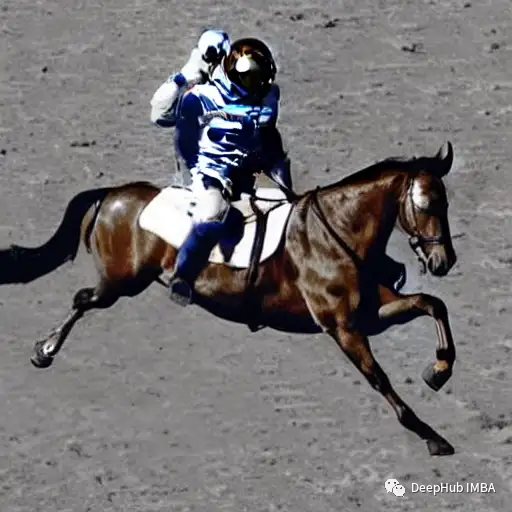
Another parameter is the Guidance Scale. This is a way to improve adherence to the conditional signal, which in the case of diffusion models is the text and overall sample quality.
Simply put, non-classified information guidance forces the generation to better match the text prompt. Numbers like 7 or 8.5 can yield good results. If a very large number is used, the image may look good but will reduce diversity.
If you want to generate multiple images for the same text prompt, simply repeat the input text multiple times. We can send a list of texts to the model; let’s write a helper function to display multiple images.
from PIL import Image def image_grid(imgs, rows, cols): assert len(imgs) == rows*cols w, h = imgs[0].size grid = Image.new('RGB', size=(cols*w, rows*h)) grid_w, grid_h = grid.size for i, img in enumerate(imgs): grid.paste(img, box=(i%cols*w, i//cols*h)) return gridNow, we can generate multiple images and display them together.
num_images = 3 prompt = ["a photograph of an astronaut riding a horse"] * num_images images = pipe(prompt).images grid = image_grid(images, rows=1, cols=3) grid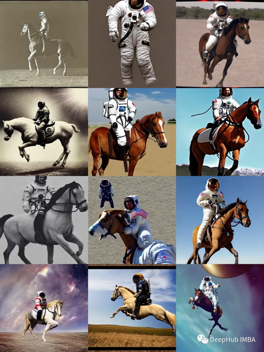
You can also generate n*m images:
num_cols = 3 num_rows = 4 prompt = ["a photograph of an astronaut riding a horse"] * num_cols all_images = [] for i in range(num_rows): images = pipe(prompt).images all_images.extend(images) grid = image_grid(all_images, rows=num_rows, cols=num_cols) grid
The generated images are by default 512*512 pixels. You can use the height and width parameters to change the height and width of the generated images. Here are some tips for choosing good image sizes:
Both height and width parameters should be chosen as multiples of 8. Setting both height and width to less than 512 may lead to poorer quality, and if both are set to more than 512, global coherence may occur. Therefore, if larger images are needed, try fixing one value at 512 while the other is greater than 512. For example, the following sizes:
prompt = "a photograph of an astronaut riding a horse" image = pipe(prompt, height=512, width=768).images[0] image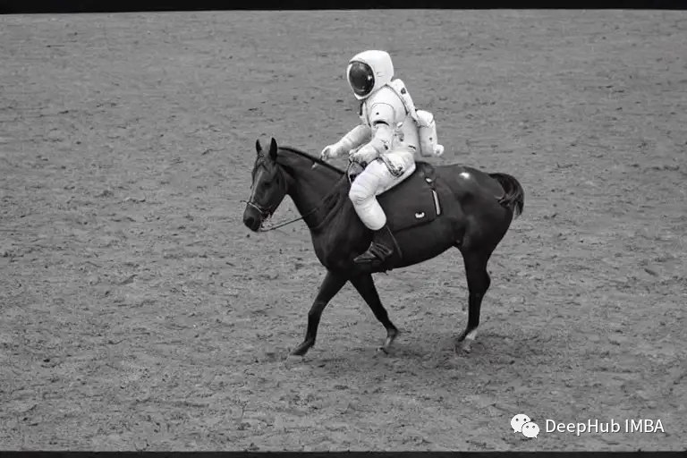
Building Your Own Processing Pipeline
We can also customize the diffusion pipeline with the Diffusers library. Here, we will demonstrate how to use a different scheduler, namely Katherine Crowson’s K-LMS scheduler.
Let’s first look at the StableDiffusionPipeline:
import torch torch_device = "cuda" if torch.cuda.is_available() else "cpu"The pre-trained model includes all the components needed to build a complete pipeline. They are stored in the following folders:
text_encoder: Stable Diffusion uses CLIP, but other diffusion models may use other encoders like BERT.
tokenizer: It must match the tokenizer used by the text_encoder model.
scheduler: The scheduler algorithm used to gradually add noise to the image during training.
U-Net: The model used to generate the latent representation of the input.
VAE, which we will use to decode the latent representation into real images.
Components can be loaded by referencing the folder where they are saved, using the subfolder parameter of from_pretrained.
from transformers import CLIPTextModel, CLIPTokenizer from diffusers import AutoencoderKL, UNet2DConditionModel, PNDMScheduler # 1. Load the autoencoder model which will be used to decode the latents into image space. vae = AutoencoderKL.from_pretrained("CompVis/stable-diffusion-v1-4", subfolder="vae") # 2. Load the tokenizer and text encoder to tokenize and encode the text. tokenizer = CLIPTokenizer.from_pretrained("openai/clip-vit-large-patch14") text_encoder = CLIPTextModel.from_pretrained("openai/clip-vit-large-patch14") # 3. The UNet model for generating the latents. unet = UNet2DConditionModel.from_pretrained("CompVis/stable-diffusion-v1-4", subfolder="unet")Now, instead of loading the predefined scheduler, we will load K-LMS:
from diffusers import LMSDiscreteScheduler scheduler = LMSDiscreteScheduler(beta_start=0.00085, beta_end=0.012, beta_schedule="scaled_linear", num_train_timesteps=1000)Move the models to GPU.
vae = vae.to(torch_device) text_encoder = text_encoder.to(torch_device) unet = unet.to(torch_device)Define parameters for generating images. Compared to the previous example, set num_inference_steps = 100 to obtain clearer images.
prompt = ["a photograph of an astronaut riding a horse"] height = 512 # default height of Stable Diffusion width = 512 # default width of Stable Diffusion num_inference_steps = 100 # Number of denoising steps guidance_scale = 7.5 # Scale for classifier-free guidance generator = torch.manual_seed(32) # Seed generator to create the initial latent noise batch_size = 1Get the text embeddings for the text prompt. Then use the embeddings to condition the U-Net model.
text_input = tokenizer(prompt, padding="max_length", max_length=tokenizer.model_max_length, truncation=True, return_tensors="pt") with torch.no_grad(): text_embeddings = text_encoder(text_input.input_ids.to(torch_device))[0]Obtain unconditional text embeddings for classifier-free guidance, which are just the embeddings of padding tokens (empty text). They need to have the same shape as text_embeddings (batch_size and seq_length).
max_length = text_input.input_ids.shape[-1] uncond_input = tokenizer( [""] * batch_size, padding="max_length", max_length=max_length, return_tensors="pt" ) with torch.no_grad(): uncond_embeddings = text_encoder(uncond_input.input_ids.to(torch_device))[0]For classifier-free guidance, two forward passes need to be performed. The first is the conditional input (text_embeddings), and the second is the unconditional embeddings (uncond_embeddings). Concatenate both into a single batch to avoid performing two forward passes:
text_embeddings = torch.cat([uncond_embeddings, text_embeddings])Generate initial random noise:
latents = torch.randn( (batch_size, unet.in_channels, height // 8, width // 8), generator=generator, ) latents = latents.to(torch_device)The generated shape is a random latent space of size 64 * 64. The model will convert this latent representation (pure noise) into a 512 * 512 image.
Initialize the scheduler with the selected num_inference_steps. This will compute the sigma and the exact step values used in the denoising process:
scheduler.set_timesteps(num_inference_steps)K-LMS requires multiplying the latent space value by its sigma:
latents = latents * scheduler.init_noise_sigmaFinally, the denoising loop:
from tqdm.auto import tqdm from torch import autocast for t in tqdm(scheduler.timesteps): # expand the latents if we are doing classifier-free guidance to avoid doing two forward passes. latent_model_input = torch.cat([latents] * 2) latent_model_input = scheduler.scale_model_input(latent_model_input, t) # predict the noise residual with torch.no_grad(): noise_pred = unet(latent_model_input, t, encoder_hidden_states=text_embeddings).sample # perform guidance noise_pred_uncond, noise_pred_text = noise_pred.chunk(2) noise_pred = noise_pred_uncond + guidance_scale * (noise_pred_text - noise_pred_uncond) # compute the previous noisy sample x_t -> x_t-1 latents = scheduler.step(noise_pred, t, latents).prev_sampleThen, using the VAE, we can decode the generated latent space back into images:
# scale and decode the image latents with vae latents = 1 / 0.18215 * latents with torch.no_grad(): image = vae.decode(latents).sampleFinally, convert the image to PIL so we can display or save it.
image = (image / 2 + 0.5).clamp(0, 1) image = image.detach().cpu().permute(0, 2, 3, 1).numpy() images = (image * 255).round().astype("uint8") pil_images = [Image.fromarray(image) for image in images] pil_images[0]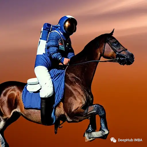
This completes the processing pipeline of a complete Stable Diffusion model. After reading this article, I hope you now know how to use Stable Diffusion and understand how it works. If you have further questions about its processing pipeline, you can delve deeper into its workflow by customizing the processing pipeline. I hope this article is helpful to you.
