Introduction and Practice of GAN

Generative Adversarial Networks (GAN) is a generative model proposed by OpenAI researcher Ian Goodfellow in 2014. Since its introduction, it has received widespread attention and research in the field of deep learning. Currently, GANs can be found in image generation, style transfer, image transformation, image description, unsupervised learning, and even reinforcement learning. GAN primarily addresses generative problems. The field of deep learning can be divided into two main categories: one is detection and recognition, such as image classification and object recognition, which mainly use models like VGG, GoogLeNet, and Residual Networks. Almost all networks are based on recognition; the other is image generation, which solves the problem of how to generate images from some data. Generative models mainly include Deep Belief Networks (DBN) and Variational Autoencoders (VAE). To some extent, GANs far exceed DBN and VAE in generative capability. Improved GANs can generate images that are indistinguishable from real ones. This article will first introduce some principles and formula derivations of GANs, and will also provide a detailed implementation of GAN image generation using TensorFlow, based on Python.

GAN mainly solves generative problems, specifically how to generate images from a segment of arbitrary random numbers. Assume a 100-dimensional vector X{x1, x2,…, x100} is given as the input to the network, where x is a random number generated, usually following a Gaussian or uniform distribution. Through adversarial training, GAN can generate clear images. This process is achieved by GAN continuously simulating the pixel distribution of images in the training set. After reading the principles of GAN below, you may have a clear understanding of this process.

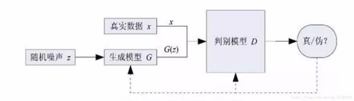
Figure 1

First, here is a flowchart of the GAN network, as shown in Figure 1. Unlike traditional discriminative network models, GAN consists of two network models: a generative model G (generator) and a discriminative model D (discriminator), where D is the network commonly used in detection and recognition models. The general process of GAN is that G takes random noise as input to generate an image G(z), regardless of the quality of the generated image. Then D takes G(z) and the real image x as input, performing a binary classification to determine which is the real image and which is the generated fake image. The output of D is a probability value; for example, if D outputs 0.15 when G(z) is the input, it means D believes there is a 15% chance that G(z) is a real image. G and D will continuously improve themselves based on D’s output; G increases the similarity between G(z) and x to deceive D as much as possible, while D will learn to avoid being deceived by G. The two engage in a zero-sum game, which can be described by a simple example: we can think of G as a counterfeiting gang and D as the police. G continuously produces fake currency, while D’s task is to distinguish G’s fake currency from real money. Initially, G lacks experience and produces poor-quality fake currency, making it easy for D to identify. Thus, G continually improves its techniques, producing increasingly realistic counterfeits, making it harder for D to distinguish between real and fake. After many iterations of this cycle, G’s fake currency can become indistinguishable from real currency, and D finds it difficult to tell the difference. Correspondingly, in image generation, G can generate images that a typical classification neural network cannot distinguish as real or fake, thus gaining the ability to generate images.

The interesting point that differs from traditional neural network training is that the training method for the generator is different; the updates to the generator’s parameters come from the backpropagated gradients of D. The generator’s goal is to “fool” the discriminator. Using game theory analysis techniques, it can be proven that there exists a Nash equilibrium in this process.

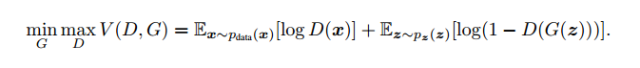
Here is the definition of their loss function, which is actually a cross-entropy. The goal of the discriminator is to make D(x) as close to 1 as possible and D(G(z)) as close to 0 as possible, so D mainly maximizes the above loss function, while G does the opposite, primarily minimizing the loss function.

Training Process:

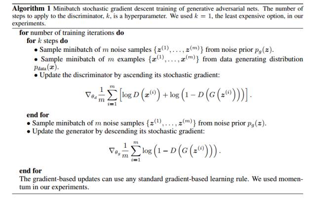
(Figure 2)

Figure 2 shows the pseudocode for GAN training. First, within the range of iteration counts, a batch of z and x is sampled to obtain their data distributions. Then, using stochastic gradient descent, D is updated k times, followed by one update for G. This approach ensures that D always has sufficient capability to distinguish between real and fake. In practice, we may update G several times for every one update of D; otherwise, if D learns too well, it can lead to the vanishing gradient problem in the early stages of training.

Before seeking a balance point, we first make a mathematical assumption, that is, under the fixed G, the optimal form of D is determined, and then we observe the problem of G minimizing the loss function based on D’s optimal form.

Assuming under the condition of fixed G, we can simplify the loss function as follows:

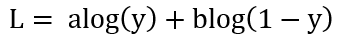
The goal of D is to maximize L. By taking the derivative of L and setting the derivative to 0, we can calculate the value of y when L reaches its maximum:

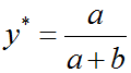
Thus, the optimal solution for D can be expressed as:

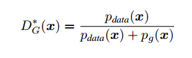
Here we conclude that when G is fixed, the optimal form of D is as shown above.

Next, we need to find out what form G must take to minimize the loss function when D is optimal to achieve a balance point between the two.

Substituting into the loss function, it can be expressed as follows:

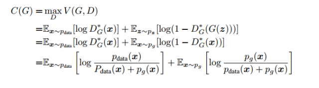
At this point, we observe that the expression is still in the form of cross-entropy, also known as KL divergence, which is often used to measure the distance between distributions and is asymmetric. Similarly, there is another divergence used to measure the distance between data distributions—JS divergence, and they have the following relationship.

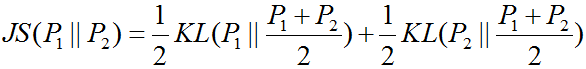
However, JS divergence has an important property: it is always greater than or equal to 0, and achieves the minimum value of 0 only when P1=P2.

Thus, we can express C(G) in terms of JS divergence:

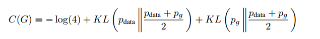
That is, C(G) achieves its minimum value of -log(4) if and only if Pg=Pdata, meaning that when D is optimal, G can minimize the loss function to -log(4), and at the minimum point Pg=Pdata, the distribution of real data equals the distribution of generated data.

At this point, it is intuitively clear that Pg=Pdata means D is exactly 0.5, meaning D has a 50% chance of thinking D(G(z)) is real data and a 50% chance of thinking it is fake data, which is akin to flipping a coin. This also indicates that the data generated by G is sufficiently indistinguishable from real data.

Thus, we have completed the introduction to the principles and mathematical derivation of GAN. Theoretically, it shows that as long as GAN is trained properly, G can perfectly simulate the data distribution and generate real images. However, during the mathematical derivation, we made some assumptions for convenience, and in practice, GAN faces training difficulties, gradient vanishing, and mode collapse issues, which will not be emphasized here.

First, create a train.py file and establish a class named Train within it, performing some initializations in the class’s constructor:

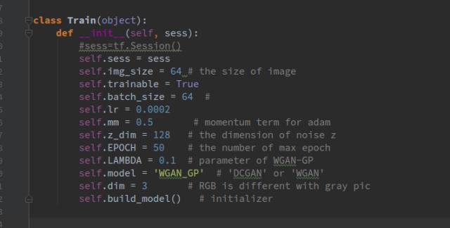
The Self.build_model() function is used to store the code for constructing the flow graph, which will be introduced later, while the other initializations are simple parameters.

Next, we will introduce the networks for the generator and discriminator:

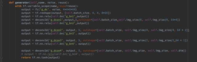
The generator takes three parameters: name, input data, and a boolean state variable reuse, indicating whether the generator is reused (reuse=True) or not (reuse=False).

The generator consists of 1 fully connected layer and 4 transposed convolutional layers, each followed by a batch normalization layer, using ReLU as the activation function. The functions fc(), deconv2d(), and bn() are our encapsulated functions representing fully connected layers, transposed convolutional layers, and normalization layers, respectively, as shown below:

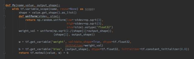
The input parameter value for the fully connected layer fc represents the input vector, while output_shape indicates the dimension of the output vector after passing through the fully connected layer. For instance, in our generator, the noise vector dimension is 128, and we output a dimension of 4*4*8*64.

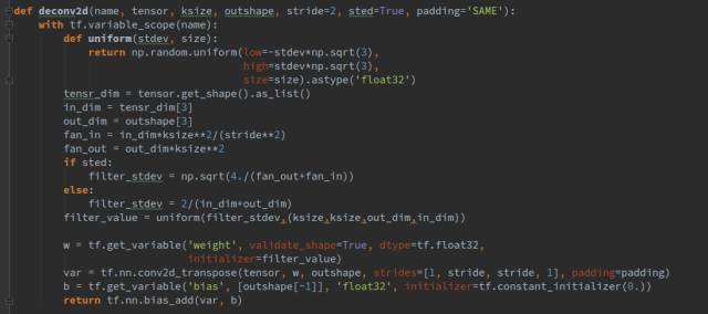
Here, Ksize refers to the size of the convolution kernel, outshape indicates the shape of the output tensor, and sted is a boolean parameter indicating whether to initialize parameters in different ways.

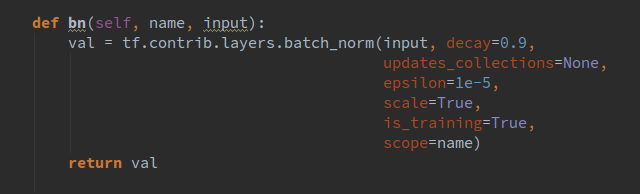
The bn() function is defined directly within the train class, as shown below:

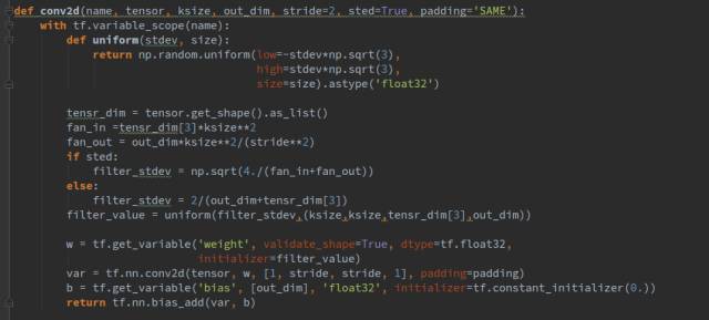
We hope the weights can be initialized to a relatively good value, so I did not use a fixed variance Gaussian distribution for initialization, but calculated a suitable variance based on the different input and output channel counts of each layer. Similarly, we have encapsulated the convolution operation, as shown below:

Now that we have introduced the structure of the generator and some basic functions, let’s introduce the discriminator network, with the code shown below:

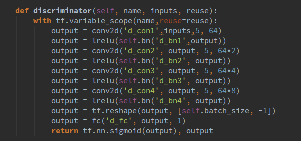
Unlike the generator, we use leaky ReLU as the activation function.

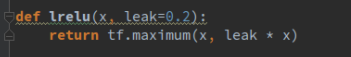
The definitions of these functions are placed in the layer.py file.

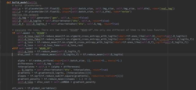
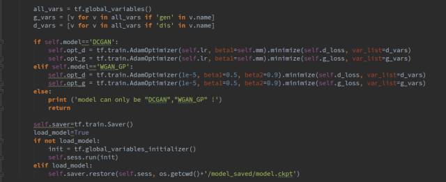
There are two GANs to choose from: DCGAN and WGAN-GP. The only difference between them is the calculation of the loss function; the network structure is the same. Both are improved versions of GAN, with WGAN-GP performing better. DCGAN often encounters training stability issues.

At this point, we have covered all the initialization processes. Next is the data extraction and network training portion. For training data, we use the CelebA dataset, which contains around 200,000 images. The sizes of the images in the dataset are not uniform, so we can use a small piece of code to crop the faces from the images and resize them to 64*64.

The code is as follows:

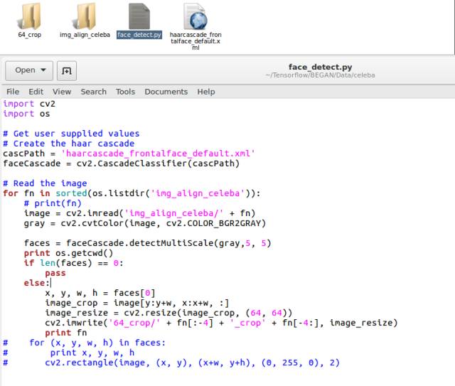
After downloading the dataset and extracting it into the img_align_celeba folder, run face_detec.py, and the cropped images will be placed in the 64_crop folder. Originally, there were 200,000 images, but after cropping, only 150,000 remain.

Next is the training part. First, we read the data; the load_data() function reads a batch_size of data each time as input to the network. During training, we choose to train D once and G twice, rather than training D multiple times before training G, as that can lead to training instability. If D learns too well, it easily distinguishes real from fake, making it difficult for G to improve, which can discourage G’s generating enthusiasm.

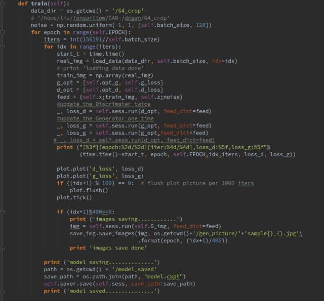
The Plot() function will plot the network loss changes after every 100 steps of training, and this is another encapsulated function.

We also choose to generate an image every 400 steps of training to observe the generator’s performance.

In the load_data() function, we did not use queues or convert to record files for reading, which would certainly be faster. We use scipy.misc to read the images.

Specifically, it is import scipy.misc as scm

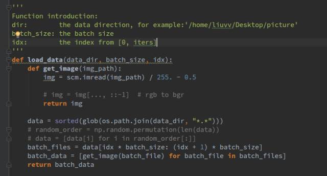
As we can see, we first sort all the images and return a list that stores the index positions of each image. This way, we can load a batch_size of data into memory each time, and the loaded data undergoes normalization, which we choose to normalize to [-0.5, +0.5].

Next is the result display, where the changes in training loss are shown as follows:

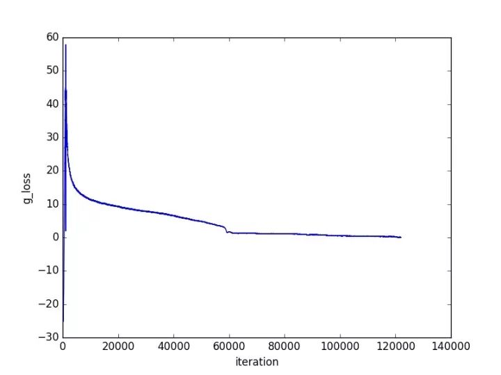
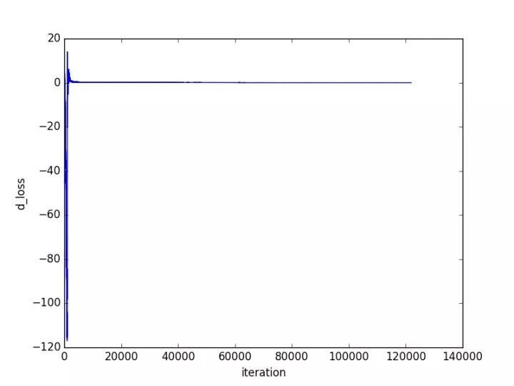
As shown in the figures, after a large fluctuation, the network converges quite well.

Next is to display the generated results:

When I tested, I set the batch_size to 16:

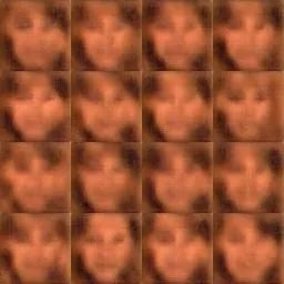
When training for 1 epoch, it looked like this:

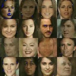
After training for a while:

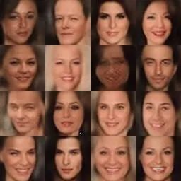
Further training seemed to result in worse outcomes, and it was evident that the model did not learn the features of glasses (the second one in the last row), likely because there were fewer images of glasses in the dataset. However, the features of eyes, nose, and mouth were learned quite well.

Results of failed training:

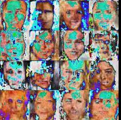
Now, let me share my experiences in training GANs. GANs are incredibly difficult to train. Even when using WGAN and WGAN-GP, I still encountered training difficulties. The results presented above are derived from multiple experiments. Some of the generated results during the experiments were truly terrible, as shown below. I summarized a few reasons: one reason is that the network structure is too simple. The network I used this time is the DCGAN structure, which was popular several years ago, and there is significant room for improvement. It is not commonly used now. I also tried BEGAN, which is indeed much easier to train; as long as you write the code well, you can let it run on its own without issues, and it performs quite well. Another reason is the choice of optimizer and the settings of hyperparameters like learning rate. Properly set hyperparameters are very helpful for GAN training. As for the optimizer, it is best to avoid using SGD, as the balance point of GAN is a saddle point, where the gradient is nearly zero. Using gradient-based optimization methods makes it difficult to converge to the optimal point. Additionally, SGD training oscillates, which can easily lead to training instability. Theoretically, this is the case, but the actual issues are much more complex.