Data Augmentation and Prediction of Food Processing Contaminants

1 Data Augmentation Based on the TimeGAN Model

Accurate prediction of contaminants in the food processing process requires a large amount of data for model training. Therefore, the TimeGAN method, which is suitable for augmenting contaminant data in the food processing process based on “temporal dynamics,” is used to augment small sample contaminant data while retaining its temporal relevance. TimeGAN was proposed in 2019 as a GAN-based framework that can generate real time series data from various fields. Unlike other GAN architectures that achieve unsupervised adversarial loss on real and synthetic data, the TimeGAN architecture introduces the concept of supervised loss to encourage the model to capture the temporal conditional distribution of data by using the original data as supervision.

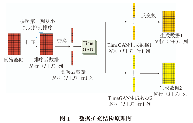
First, the original data is sorted by the size of the first stage contaminant and compressed into one-dimensional data, which is then input into TimeGAN. Through learning from the original data, TimeGAN generates multiple sets of data. These generated data are similar to the original data, and finally, the generated one-dimensional data is resized to match the dimensions of the original data. Sufficient generated data can be obtained according to demand to meet the data volume required for deep learning training.

Let the number of processing stages be I + J, where I is the number of stages with known contaminant concentrations, and J is the number of stages for which contaminant concentrations need to be predicted. The contaminant data in the food processing process is defined as shown in Equation (1):

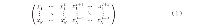
In the equation, N is the number of sample data, at this time the data size is N × (I + J).

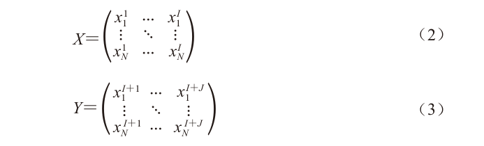
Dividing Equation (1), let the data of the stages with known contaminant concentrations be X, and the data of the stages with contaminant concentrations that need to be predicted be Y, as shown in Equations (2) and (3):

Considering that the contaminant data in the food processing process changes in the row direction according to the number of stages, while in the column direction it is another set of samples, the trend of the relationship between two rows of data remains the same. However, the initial data value of the tth row data (where t = 1, 2…N) differs, leading to different subsequent stage values (where h = 2, 3…I + J), but still related to . Therefore, there is also a certain variation pattern between each column of data, so the “temporal dynamics” relationship described by TimeGAN is the relationship between each set of data. Thus, data preprocessing must be performed before inputting the data into the TimeGAN model.

The structure diagram of the TimeGAN model for augmenting contaminant data in the food processing process is shown in Figure 1. First, the original data is sorted by the size of the first stage contaminant, and the corresponding subsequent stages are also rearranged accordingly, resulting in sorted N rows (I + J) of data, which are all treated as a set of data. The transformed data becomes N × (I + J) one-column one-dimensional data, which is then input into TimeGAN. Through learning from the original data, TimeGAN generates multiple sets of generated data. Finally, the generated one-dimensional data is inversely transformed to restore it to the same N rows (I + J) of data as the original data. These generated data are similar to the original data but differ, and multiple sets of data can be generated until there is enough data for the prediction model training.

2 Prediction of Contaminants in the Food Processing Process Based on GAN and DF Models

GAN consists of a generator and a discriminator. The generator learns to produce generated data similar to real data, while the discriminator’s role is to distinguish between real data and data generated by the generator, reflecting the idea of competitive learning. The generator and discriminator compete with each other for optimization learning, and after learning, the data generated by the generator is very realistic, achieving the goal of being indistinguishable from the real.

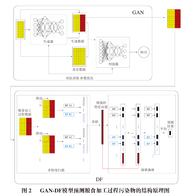
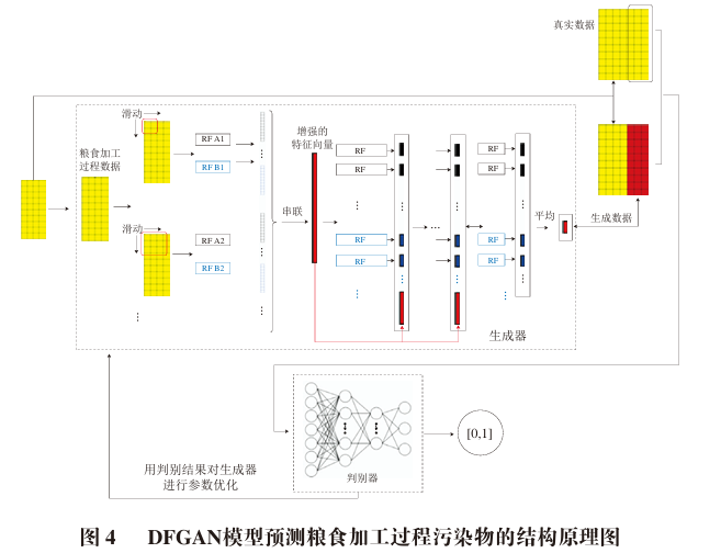
To enable the generator of GAN to predict contaminants in the food processing process, the generator is designed to input known stages of contaminant data in the food processing process and output the contaminant data for the stages that need to be predicted. Based on the structure of GAN, DNN is used. The input of the GAN generator is the known I stages, which then pass through four layers of DNN networks, ultimately obtaining the J stages that need to be predicted. The input to the discriminator of GAN is the (I + J) stages, which also pass through four layers of DNN networks, outputting a one-dimensional scalar and finally obtaining the classification result through an activation function.

The GAN is combined with DF, first using GAN for prediction. The known I stages and the J stages predicted by GAN are fused.

The output of the GAN model for X_train is defined as . Its data size is the same as that of Y_train. When there are N groups of data, is of size N rows by J columns. The trained input X_train and output Y_train data are used to train GAN. The trained GAN model can obtain from X_train, merging X_train with , keeping the row count unchanged and merging the column count.

The merged data becomes N rows and (I + J) columns, and the merged data serves as the input to DF, obtaining the J stages predicted by GAN. Here, DF not only learns the variation relationship between the known I stages and the predicted J stages but also learns the deviation of the GAN prediction results, further improving prediction accuracy.

During the training of the GAN-DF model, each training data set is first used to train GAN. After GAN is trained, the results predicted by GAN for the training set are fused with the training set inputs, and the fused inputs are used as the inputs for the DF training set, combined with the training set outputs to train DF. After DF learns the variation patterns of food contaminant processing and the errors of GAN predictions through training, the GAN-DF model is obtained. Then, test data is used to compute the accuracy of the model predictions.

X_train and Y_train are used for the first training of DF. After training, the DF model can obtain the prediction value from X_train. The horizontal merge of X_train and results in the input for the discriminator . This is generally represented as Equation (4):

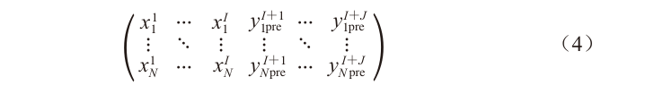
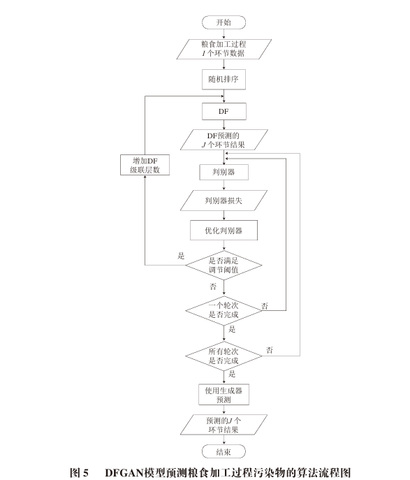
In the equation, is the predicted value for the Nth group of data at the (I + J)th stage. Since ‘s (I + 1)th to (I + J)th stage data is predicted by DF, so the discriminator needs to label it as false, thus assigning the label 0. Meanwhile, the input combined with the output of the test set, i.e., the data shown in Equation (1), is real data, so it is labeled 1 and input into the discriminator. Based on the effectiveness of the discriminator’s judgment, backpropagation is performed for optimizing the discriminator with the loss function being BCE Loss. Since the generator cannot directly use the discriminator’s results for backpropagation training, the discriminator’s loss function is used to evaluate the performance of the generator, checking the current prediction accuracy of the generator for the training data. If the loss function of the discriminator relative to the previous adjustment of the generator’s loss function has not changed, it indicates that the generator’s prediction performance is still good, and optimization of the generator is not needed. If the loss function relative to the previous adjustment has changed, and the absolute value of the change reaches the adjustment threshold, then the generator is adjusted, increasing the number of cascaded layers, with the adjustment threshold defined as shown in Equation (5):

In the equation, δ_e is the absolute value of the current prediction error minus the previous prediction error; epoch is the current training round. The design idea of δ_e is that at the beginning of training, epoch is small, and the prediction effect changes significantly as epoch increases. At this time, it is hoped that δ_e is large, allowing for rapid increases in cascaded layers. When epoch is relatively large, the prediction effect changes less with increasing epoch, and it is hoped that δ_e remains small, allowing for minor adjustments in the number of cascaded layers. Even when epoch is very large, δ_e should still have a certain value. The initial value of δ_e is defined as 0. Therefore, the adjustment threshold defined by Equation (5) is such that δ_e is a value that decreases as epoch increases, where a needs to be determined based on the magnitude of prediction accuracy; b is a factor affecting the decay rate of δ_e, with values typically between 0.8 and 0.99; c is set to ensure that even when the number of training rounds is large, δ_e still has a certain value. When the size of δ_e reaches the adjustment threshold, it indicates that the previous adjustment of the generator in increasing the number of cascaded layers has resulted in a significant change in prediction performance, and optimization of the generator is still required until all batches of training are completed.

As shown in Figure 5, the model is initialized first. At the beginning of each training round, it checks whether the size of δ_e reaches the adjustment threshold. If it does, the number of layers in the cascaded forest of the generator is increased by one, and the generator is trained with the training data. Then, the discriminator is trained for this round. In this round of training, each batch of samples is input into the generator for prediction, while real data is used to train the discriminator. After this round of training, the size of δ_e is checked again, and this process is repeated until the round ends.

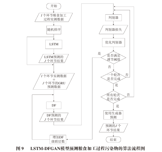
To further improve prediction accuracy, a prediction model based on Long Short-Term Memory (LSTM)-DFGAN is established.

First, the LSTM-DF model is established, defining as the output of the LSTM model for X_train, which has the same data size as Y_train. When there are N groups of data, is of size N rows by J columns. The training input X_train and output Y_train data are used to train the LSTM. The trained LSTM model can obtain from X_train, merging X_train with results in the input for DF, which has N rows and (I + J) columns. This data serves as the input for DF, while Y_train serves as the output for DF. The DF is trained using these inputs and outputs to learn the variation patterns of food contaminants and the errors in LSTM predictions, resulting in the LSTM-DF model structure shown in Figure 6.

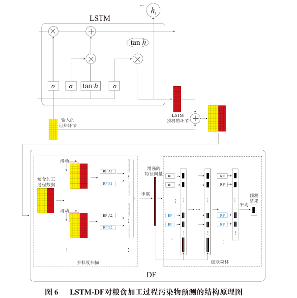
After data partitioning, the input and output data of the training set are obtained. Each training data set is first used to train LSTM. After LSTM is trained, the prediction results of LSTM for the training set are fused with the training set inputs. The fused input is then used as the input for the DF training set, combined with the training set outputs to train DF. After DF learns the variation patterns of food contaminants and the errors in LSTM predictions through training, the LSTM-DF model is obtained.

3 Model Simulation and Validation

The dataset includes 12 types of rice models from Jiangsu, Hubei, Heilongjiang, etc., encompassing five heavy metal contaminants: lead (Pb), chromium (Cr), arsenic (As), cadmium (Cd), and mercury (Hg), with a total of 84 sample groups. Taking lead (Pb) as an example, the proposed methods for augmenting and predicting contaminant data in the food processing process are validated. The four-layer DNN networks involved in the GAN network all use two hidden layers of sizes 512 and 256, with the number of network nodes in the input layer equal to the input data size and the output layer nodes equal to the output data size.

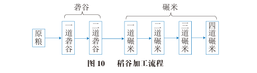
Figures 11 to 14 show the results of augmenting the original data into 1, 10, 100, and 1000 groups, where each group size is 12×7, corresponding to the 12 types of rice models and 7 processing techniques.

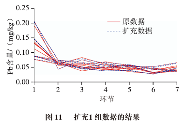
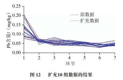
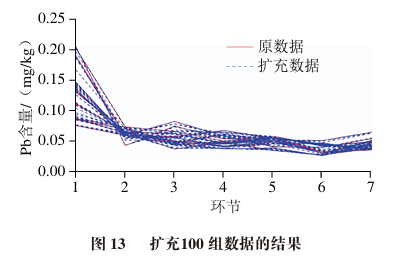
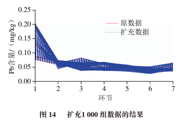
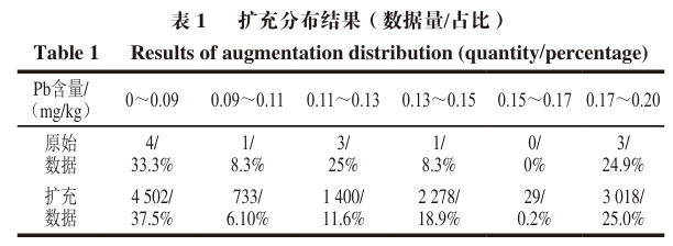
To verify the effectiveness of the original data and generated data, some statistical validations are performed, including centroid comparison and data distribution intervals.

The centroid of each stage data for the original data is calculated as [0.12, 0.06, 0.05, 0.05, 0.04, 0.03, 0.04], while the generated data centroid is [0.13, 0.06, 0.05, 0.05, 0.05, 0.03, 0.04].

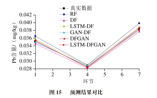
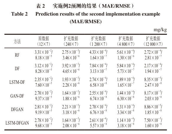
In summary, from the perspective of different models, the LSTM-DFGAN model has the smallest error, followed by the GAN-DF model, then the LSTM-DF model and the DFGAN model. The errors of these four models are generally in the same order of magnitude and have small differences. The largest errors are from the RF model and the DF model, with errors approximately 2-3 times higher than the previous three models. The DF performs better with larger data volumes, while RF performs better with smaller data volumes. This demonstrates that the LSTM-DFGAN model proposed in this paper has excellent prediction performance and can effectively predict contaminants in the food processing process.

From the perspective of data augmentation, the prediction effects of the original data are poor due to the small data volume, which leads to a high risk of overfitting. As the amount of data augmentation increases, the prediction effects of each model improve. The increase in data volume brings greater prediction improvements for LSTM-DF, GAN-DF, DFGAN, and LSTM-DFGAN, improving by about three orders of magnitude, while the prediction accuracy improvement for RF and DF is relatively small, around two orders of magnitude.

Conclusion

This experiment addresses the augmentation of small sample data for contaminants in the food processing process and the prediction of contaminants in this intermittent process by introducing TimeGAN, a time series data generation technology in the field of deep learning, and discrete time series modeling and prediction technology. By improving and combining the unsupervised learning GAN model, the DF model suitable for discrete process modeling, and the LSTM model for time series prediction, models such as GAN-DF, DFGAN, and LSTM-DFGAN are established, proposing a novel algorithm suitable for data augmentation and prediction of contaminants in the food processing process. Through simulation validation of metal contaminant data in the rice processing process, the results indicate that the TimeGAN method for data augmentation is feasible, and the LSTM-DFGAN model demonstrates the most ideal overall prediction effect. This research belongs to the intersection of food and artificial intelligence, possessing certain theoretical and practical innovations in the direction of intelligent prediction for food safety. The research results can improve the accuracy and effectiveness of predicting contaminants in the food processing process, significantly reducing the incidence of contamination during food processing, and positively contributing to food safety and the interdisciplinary development of related fields.