This article mainly summarizes the notes from the CS231n course, adding knowledge from the Deep Learning Book and practical TensorFlow, as well as the Caffe framework.
1. Convolutional Neural Networks
1.1 Convolutional Neural Networks vs. Conventional Neural Networks
1.1.1 Similarities
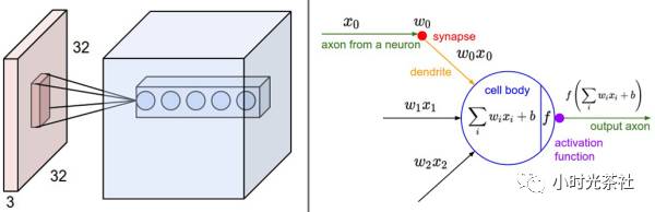
Convolutional networks are a type of neural network specifically designed to process data with a grid-like topology. They are very similar to conventional neural networks: both consist of neurons, which have learnable weights and biases. Each neuron receives some input data, performs an inner product operation, and then applies an activation function. The entire network is still a differentiable scoring function: the input is raw image pixels, and the output is scores for different categories. In the last layer (often a fully connected layer), the network still has a loss function (such as SVM or Softmax), and various techniques and key points we implement in neural networks still apply to convolutional neural networks.
1.1.2 Differences
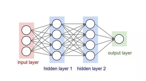
The structure of convolutional neural networks is based on the assumption that the input data is images. Based on this assumption, we add some unique properties to the structure. These unique attributes make the forward propagation function more efficient and significantly reduce the number of parameters in the network. In conventional neural networks, the input is a vector, which is transformed through a series of hidden layers. Each hidden layer consists of several neurons, each connected to all neurons in the previous layer. However, in a hidden layer, the neurons are independent of each other and do not connect.
Conventional neural networks perform poorly with large images. In CIFAR-10, the image size is 32x32x3 (32 pixels in width and height, with 3 color channels), so in the corresponding conventional neural network’s first hidden layer, each fully connected neuron has 32x32x3=3072 weights. This number seems acceptable, but it is clear that this fully connected structure is not suitable for larger images. For example, an image of size 200x200x3 will result in neurons containing 200x200x3=120,000 weight values. And since there are definitely more than one neuron in the network, the number of parameters will increase rapidly! Clearly, this fully connected method is inefficient, and a large number of parameters can quickly lead to overfitting.
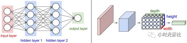
Convolutional neural networks adjust their structure to be more reasonable when the input consists entirely of images, gaining significant advantages. Unlike conventional neural networks, the neurons in each layer of a convolutional neural network are arranged in three dimensions: width, height, and depth (where depth refers to the third dimension of the activation data, not the depth of the entire network, which refers to the number of layers). We will see that the neurons in a layer will only connect to a small region of the previous layer, rather than using a fully connected approach. The following diagram illustrates the differences between a conventional neural network and a convolutional neural network:
1.2 Structure of Convolutional Neural Networks
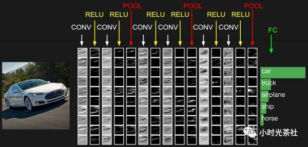
A simple convolutional neural network is composed of various layers arranged in sequence, where each layer uses a differentiable function to pass activation data from one layer to another. Convolutional neural networks mainly consist of three types of layers: convolutional layers, pooling layers, and fully connected layers (which are the same as those in conventional neural networks). By stacking these layers, a complete convolutional neural network can be constructed, as shown in the diagram below:
1.2.1 Convolutional Layer
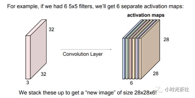
The parameters of the convolutional layer consist of a set of learnable filters. Each filter is small in spatial dimensions (width and height) but has the same depth as the input data. During forward propagation, each filter slides (or convolves) over the width and height of the input data, calculating the inner product between the filter and any location in the input data. As the filter slides over the width and height of the input data, it generates a 2D activation map, which indicates the filter’s response at each spatial location. Intuitively, the network allows the filter to learn to activate when it sees certain types of visual features, which could be edges in certain orientations or color spots in the first layer, or even honeycomb or wheel-like patterns in higher layers of the network. In each convolutional layer, we have a whole set of filters (e.g., 12), each generating a different 2D activation map. Stacking these activation maps along the depth direction generates the output data, as shown in the left diagram, where a 32*32 image is processed through multiple filters to produce output data:
(1) Local Connectivity
Local connectivity greatly reduces the number of parameters in the network. When dealing with high-dimensional inputs like images, it is unrealistic for each neuron to be fully connected to all neurons in the previous layer. Instead, we only allow each neuron to connect to a local region of the input data. The spatial size of this connection is called the neuron’s receptive field, and its size is a hyperparameter (essentially the spatial size of the filter). In the depth direction, the size of this connection is always equal to the depth of the input. It is important to emphasize that we treat the spatial dimensions (width and height) differently from the depth dimension: the connections in space (width and height) are local, while in depth, they are always consistent with the depth of the input data.
(2) Spatial Arrangement
The previous section discussed how each neuron in the convolutional layer connects to the input data, but it did not address the number of neurons in the output data and how they are arranged. There are three hyperparameters that control the size of the output data: depth, stride, and zero-padding. Below is a discussion of these:
1) Output Data Depth
This matches the number of filters used, as each filter searches for something different in the input data. For example, if the first convolutional layer’s input is the raw image, then the different neurons in the depth dimension may be activated by edges in different directions or color spots. We refer to the collection of neurons with the same receptive field arranged along the depth direction as a depth column. As shown in the diagram below, the convolutional layer has 6 filters, and the output data depth is also 6.
2) Stride
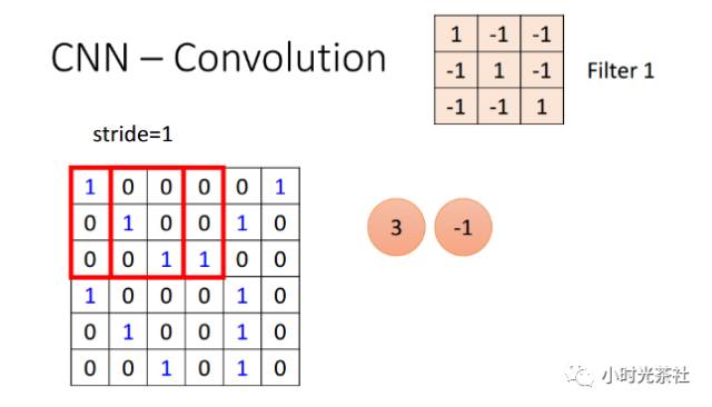
When sliding the filter, the stride must be specified. When the stride is 1, the filter moves 1 pixel at a time. When the stride is 2 (or less commonly 3 or more, which are rarely used in practice), the filter moves 2 pixels at a time. This operation will reduce the spatial size of the output data. As shown in the diagram below, when the stride is 1, the input data size is 6 * 6, and the output data size is 4 * 4.
3) Padding
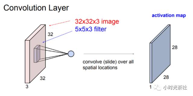
The output of the convolution layer will reduce the size of the data, as shown in the diagram below, where the input of size 32 * 32 * 3 processed by a filter of size 5 * 5 * 3 results in output data of size 28 * 28 * 1.
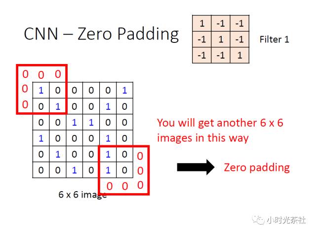
Zero-padding has a good property that it can control the spatial size of the output data (most commonly used to keep the input data’s spatial size consistent, so that the width and height of the input and output are equal). It is convenient to pad the input data with 0s at the edges, and the size of this zero-padding is a hyperparameter. The diagram below shows that zero-padding maintains the consistency of the input and output data dimensions.
Convolution Layer Output Calculation Formula:
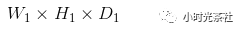
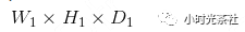
Assuming the input data size is:
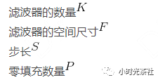
The four hyperparameters of the convolution layer are:
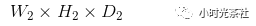
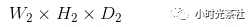
Then the size of the output data will be:
Where:
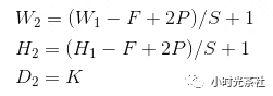
For these hyperparameters, common settings are F=3, S=1, P=1. For example, if the input is 7×7, the filter is 3×3, the stride is 1, and padding is 0, then the output will be 5×5. If the stride is 2, the output will be 3×3.
(3) Parameter Sharing
Using parameter sharing in the convolutional layer is to control the number of parameters. Each filter is locally connected to the previous layer, and all local connections of each filter use the same parameters, which also significantly reduces the number of parameters in the network.
Here, we make a reasonable assumption: if a feature is useful when computing at a certain spatial location (x,y), it will also be useful when computing at another different location (x2,y2). Based on this assumption, we can significantly reduce the number of parameters. In other words, we treat a single 2D slice in the depth dimension as a depth slice (for example, a data size of [55x55x96] has 96 depth slices, each of size [55×55]). All neurons in each depth slice use the same weights and biases. During backpropagation, we calculate the gradient of each neuron with respect to its weights, but we accumulate the gradients of all neurons in the same depth slice with respect to the weights, thus obtaining the gradient for the shared weights. Therefore, each slice only updates one set of weights.
When all weights in a depth slice use the same weight vector, the forward propagation in the convolutional layer can be seen as calculating the convolution of the neuron weights with the input data (this is where the name “convolutional layer” comes from). This is also why we always refer to these weight sets as filters (or kernels), because they convolve with the input. The diagram below dynamically shows the convolution process:
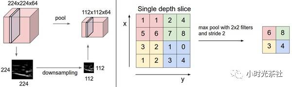
1.2.2 Pooling Layer
Typically, a pooling layer is periodically inserted between consecutive convolutional layers. Its purpose is to gradually reduce the spatial size of the data, thereby reducing the number of parameters in the network, decreasing the computational resources required, and effectively controlling overfitting. The pooling layer uses a max operation, independently processing each depth slice of the input data to change its spatial size. The most common form is for the pooling layer to use a 2×2 filter with a stride of 2 to downsample each depth slice, discarding 75% of the activation information. Each max operation takes the maximum value from four numbers (i.e., from a 2×2 area in the depth slice). The depth remains unchanged.
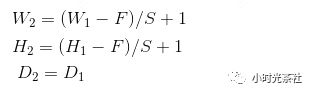
Pooling Layer Calculation Formula:
Input data size:
The pooling layer has two hyperparameters:
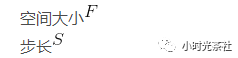
Output data size:
Where:
Since a fixed function is used to compute the input, no parameters are introduced. Zero-padding is rarely used in pooling layers.
In practice, the max pooling layer typically has two forms: one is F=3, S=2, and the other, more commonly used, is F=2, S=2. Pooling with larger receptive fields requires larger pooling sizes and is often destructive to the network.
General Pooling: In addition to max pooling, pooling units can also use other functions, such as average pooling or L-2 norm pooling. Average pooling was historically more common but is now rarely used, as practical results have shown that max pooling is more effective. The diagram below illustrates the pooling layer:
Backpropagation: To review backpropagation, the backpropagation of functions can be simply understood as passing the gradient back only through the largest number. Therefore, during forward propagation through the pooling layer, we usually record the index of the maximum element in the pool (sometimes called switches), so that during backpropagation, the routing of the gradient is very efficient.
1.2.3 Normalization Layer
In the structure of convolutional neural networks, many different types of normalization layers have been proposed, sometimes to realize the inhibition mechanisms observed in biological brains. However, these layers have gradually fallen out of favor, as practical results have shown that their effects, even when present, are extremely limited.
1.2.4 Fully Connected Layer
In the fully connected layer, neurons are fully connected to all activation data in the previous layer, just like in conventional neural networks. Their activations can be computed using matrix multiplication followed by adding a bias.
1.3 Common CNN Models
1.3.1 LeNet
This is the first successful application of convolutional neural networks, implemented by Yann LeCun in the 1990s, used for handwritten character recognition, and is the “Hello World” of learning neural networks. The network structure diagram is shown below:
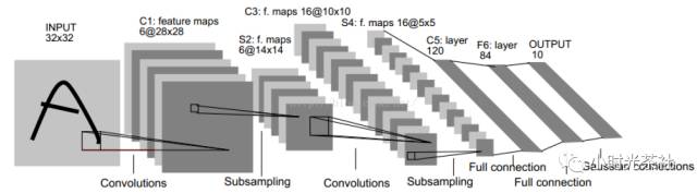
C1 Layer: Convolutional layer, which contains 6 feature convolutional kernels of size 5 * 5, resulting in 6 feature maps, each of size 32-5+1=28.
S2 Layer: This is the downsampling layer, using max pooling for downsampling, with a pooling size of 2×2, resulting in 6 feature maps of size 14×14.
C3 Layer: Convolutional layer, which contains 16 feature convolutional kernels, again of size 5×5, resulting in 16 feature maps, each of size 14-5+1=10.
S4 Layer: Downsampling layer, still using 2×2 max pooling, resulting in 16 feature maps of size 5×5.
C5 Layer: Convolutional layer, which uses 120 convolutional kernels of size 5×5, ultimately outputting 120 feature maps of size 1×1.
After this is the fully connected layer, followed by classification.
1.3.2 AlexNet
AlexNet is significant; it proved the effectiveness of CNNs under complex models, making neural networks shine in the field of computer vision. It was implemented by Alex Krizhevsky, Ilya Sutskever, and Geoff Hinton. AlexNet won the ImageNet ILSVRC competition in 2012, with performance far exceeding that of the second place (16% top-5 error rate compared to 26% for the second place). This network structure is very similar to LeNet, but deeper and larger, using stacked convolutional layers to extract features (previously, typically a single convolutional layer was used, immediately followed by a pooling layer). The structure diagram is shown below:
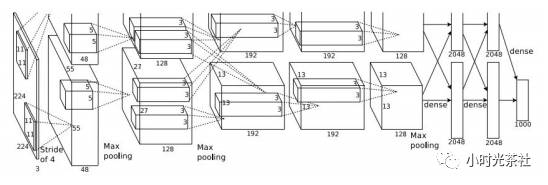
Detailed information for each layer is shown in the diagram below:
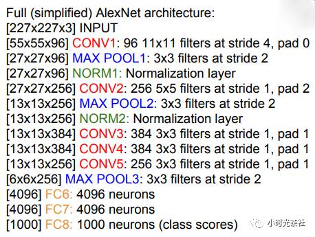
AlexNet input size is 227x227x3.
The first convolutional layer has 96 filters of size 11×11, with a stride of 4. The output size is (227 – 11) / 4 + 1 = 55, and the depth is 64. There are approximately 11x11x3x643,500 parameters.
The second layer pooling size is 3×3, with a stride of 2, resulting in an output size of (55 – 3) / 2 + 1 = 27.
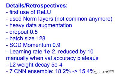
This is the first time ReLU is used, at least the first time it is popularized.
It uses data normalization, which is now not commonly used.
It employs extensive data augmentation.
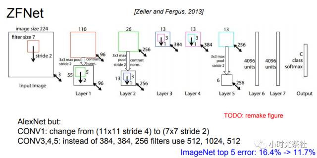
1.3.3 ZFNet
Invented by Matthew Zeiler and Rob Fergus, this network won the ILSVRC 2013 competition and is known as ZFNet (short for Zeiler & Fergus Net). It improves upon AlexNet by modifying the hyperparameters in the structure, specifically by increasing the size of the intermediate convolutional layers and making the stride and filter sizes in the first layer smaller. They made some parameter adjustments based on experiments. The structure diagram is shown below:
1.3.4 VGGNet
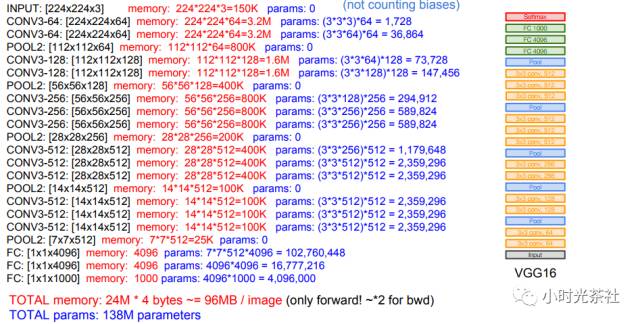
VGGNet does not make drastic architectural choices and does not do extensive work on how to set the number of filters or their sizes. The entire VGG network only uses 3*3 convolutional kernels, with a stride of 2 and 2*2 pooling windows, also with a stride of 2. This parameter setting is maintained throughout the process. The key point of VGG is the number of layers this operation is repeated; the same set of parameter settings is repeated 16 layers. The reason for choosing this number of layers may be that they found it yields the best performance. Each image requires 200M of memory, and the total number of parameters will reach 140 million.
Why use a 3*3 filter? A 3*3 filter is the smallest that can capture the receptive field of the top, bottom, left, right, and center; multiple 3*3 convolutional layers have more non-linearities than a single larger filter convolution layer. With a stride of 1, two 3*3 filters have a maximum receptive field area of 5*5, and three 3*3 filters have a maximum receptive field area of 7*7, which can replace a larger filter size. Multiple 3*3 convolution layers have fewer parameters than a single large filter, assuming the input and output feature map sizes are the same at 10, then the number of parameters in a convolution layer with three 3*3 filters is 3*(3*3*10*10)=2700, because the three 3*3 filters can be seen as a decomposition of a 7*7 filter (with non-linear decomposition in the intermediate layers), while a single 7*7 convolution layer has parameters of 7*7*10*10=4900. The 1*1 filter serves to linearly transform the input without affecting the input-output dimensions, and then undergoes non-linear processing through ReLU, enhancing the network’s non-linear expressiveness.
One downside of VGGNet is that it consumes more computational resources and uses more parameters; the structure diagram is shown below:
1.3.5 GoogLeNet
While VGGNet performs well, it has a large number of parameters. Generally, the most direct way to improve network performance is to increase the depth and width of the network, which also means a massive increase in parameters. However, a large number of parameters can easily lead to overfitting and significantly increase computational load.
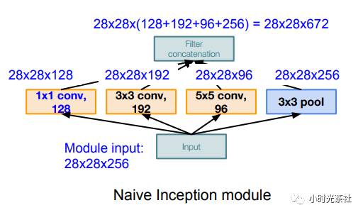
Most articles suggest that the fundamental way to solve these two drawbacks is to convert fully connected layers and even general convolutions into sparse connections. On one hand, real biological neural systems are sparsely connected; on the other hand, literature indicates that for large-scale sparse neural networks, one can construct an optimal network layer by layer through analyzing the statistical properties of activation values and clustering highly correlated outputs. The understanding of the “sparse connection structure” is to use a small and dispersed stackable network structure to learn complex classification tasks. Inception’s ability to improve network accuracy may be due to its multiple kernels of different scales, each learning different features and aggregating these features learned by different kernels for the next layer, thus achieving comprehensive deep learning.
The general Inception structure is shown in the diagram below:
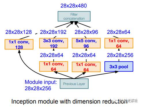
The Inception that achieves dimensionality reduction is shown in the diagram below, reducing from 256 dimensions to 64 dimensions, thus decreasing the number of parameters:
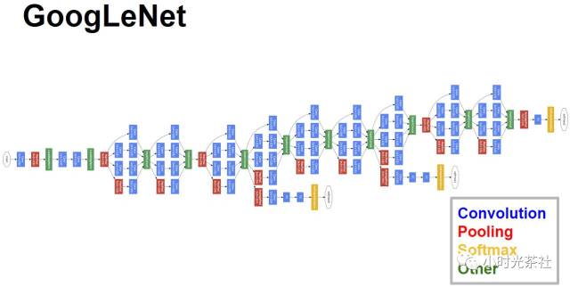
Why does VGG network have so many parameters? It is because it has two fully connected layers of 4096 at the end. Szegedy learned from this lesson, and to compress the parameters of GoogLeNet, he removed the fully connected layers. The complete structure of GoogLeNet is shown in the diagram below:
1.3.6 ResNet
Developed by Kaiming He and colleagues, the residual network not only won the ImageNet competition in 2015 but also achieved first place in many other competitions. A well-known obstacle in optimizing deep networks is the vanishing and exploding gradients. This obstacle can be mitigated through reasonable initialization and some other techniques, but as the depth of the network increases, the accuracy saturates and rapidly decreases, a phenomenon known as degradation, which is widespread in deep networks, indicating that not all systems are easy to optimize.
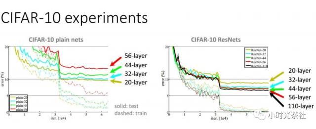
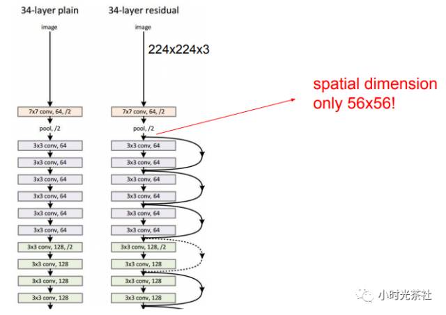
For plain networks, simply increasing the number of layers will not be effective. As shown in the diagram, on CIFAR-10, the solid line represents the error rate on the test set, while the dashed line represents the error rate on the training set. We observe that deeper networks have higher error rates, which is counterintuitive; logically, deeper networks should have greater capacity. This is because we are not optimizing the parameters well enough to select better parameters. The training error rate and test error rate of the ResNet model continue to improve as the network depth increases. Training ResNet takes 2-3 weeks on 8 GPUs.
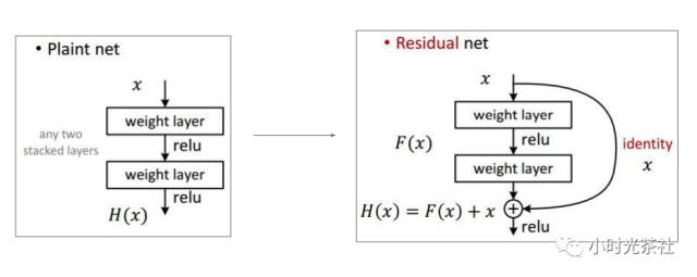
Kaiming He proposed the concept of deep residual learning to address this issue. First, we assume that the mapping we require is H(x). Through the above observations, we realize that directly obtaining H(x) is not easy, so we turn to seek the residual form F(x)=H(x)-x, assuming that obtaining F(x) is simpler than H(x). Thus, through F(x)+x, we can achieve our goal. In simple terms, the structure shown above is called a residual block. Many may have doubts about the second assumption, which is why F(x) is easier to obtain than H(x). This point is not clearly explained in the paper, but experimental results have indeed led to this conclusion.
In ResNet, there are interesting skip connections, as shown in the diagram above. In the backpropagation of the residual network, the gradient flows not only through these weights but also through these skip connections, which are additive, allowing gradients to flow back to previous parts, enabling the training of features that are close to the image.
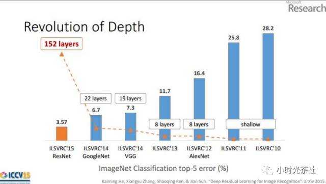
Through the diagram below showing the depth of neural network algorithms on ImageNet and their error rates, we can see that as the number of layers in the neural network increases, the error rate decreases.
2. TensorFlow Practical Implementation
2.1 Comparison of Deep Learning Open Source Frameworks
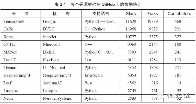
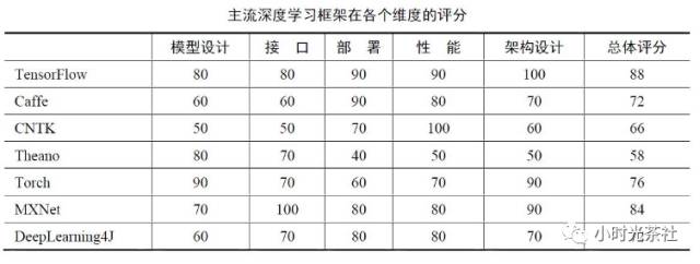
There are many deep learning frameworks; here we only introduce two that are widely used:
TensorFlow: TensorFlow is an open-source software library for numerical computation using data flow graphs, designed for machine intelligence. TensorFlow has high-quality product-level code, backed by Google’s strong development and maintenance capabilities, and its overall architecture design is excellent. As a giant company, Google invests far more resources into TensorFlow’s development than universities or individual developers, and it is foreseeable that TensorFlow’s future development will be rapid, potentially leaving behind deep learning frameworks maintained by universities or individuals. TensorFlow is a relatively high-level machine learning library, allowing users to easily design neural network structures without needing to write C++ or CUDA code for efficient implementation.
TensorFlow also has built-in upper-level components like TF.Learn and TF.Slim to help quickly design new networks. Another important feature of TensorFlow is its flexible portability, allowing the same code to be easily deployed on PCs, servers, or mobile devices with any number of CPUs or GPUs with almost no modification. In addition to supporting common network structures (Convolutional Neural Networks, CNNs, and Recurrent Neural Networks, RNNs), TensorFlow also supports deep reinforcement learning and other computationally intensive scientific calculations (such as solving partial differential equations).
Caffe: Caffe is a widely used open-source deep learning framework that was the most starred project on GitHub in the deep learning field before TensorFlow emerged. The main advantages of Caffe are: 1. It is easy to get started, as the network structure is defined in configuration files, eliminating the need to design the network through code. 2. It has fast training speeds, and its components are modular, allowing for easy expansion to new models and learning tasks. However, Caffe was initially designed only for images and did not consider text, speech, or time-series data, so its support for convolutional neural networks is excellent, but its support for time-series RNNs and LSTMs is not particularly robust.
2.2 Setting Up the TensorFlow Environment
2.2.1 Operating System
TensorFlow supports running on Windows, Linux, and Mac. The environment I set up uses Ubuntu 16.04 64-bit. TensorFlow requires a Python environment, and here I default to using Python 3.5 as the base version. It is recommended to use Anaconda as the Python environment, as it can avoid many compatibility issues.
2.2.2 Installing Anaconda
Anaconda is a scientific computing distribution of Python that comes with hundreds of commonly used libraries, some of which may be dependencies for TensorFlow. The Python version of Anaconda must match the version of TensorFlow, or there will be issues. I downloaded Anaconda3-4.2.0-Linux-x86_64.sh. Execute:
bash Anaconda3-4.2.0-Linux-x86_64.shAfter installing Anaconda, the program will prompt whether to add the Anaconda3 binary path to .bashrc; it is recommended to add it so that the python command will automatically use the Anaconda Python 3.5 environment in the future.
2.2.3 Installing TensorFlow
Tensowflow has both CPU and GPU versions. If your computer has an NVIDIA graphics card, it is recommended to install the GPU version, as it will speed up your training. The installation of the CPU version is relatively simple, so it will not be elaborated here; mainly, I will discuss the installation of the GPU version. First, use:
lspci | grep -i nvidiaTo check the model of the NVIDIA graphics card, then go to https://developer.nvidia.com/cuda-gpus to see if your graphics card supports CUDA; only CUDA-supported GPUs can install the GPU version of TensorFlow. My computer has a GeForce 940M, which supports CUDA.
(1) Installing CUDA and cuDNN
First, download the corresponding version of CUDA from the NVIDIA official website. I downloaded cuda_8.0.61_375.26_linux.run. This download may be slow, so it is recommended to use a download manager. Before installation, you need to pause the NVIDIA driver X server. First, use ctrl+alt+f2 to access the Ubuntu command interface. If you cannot enter, some computers may require using fn+ctrl+alt+f2, and then execute
sudo /etc/init.d/lightdm stopTo pause the X Server. Then execute the following command to install:
chmod u+x cuda_8.0.61_375.26_linux.run sudo ./cuda_8.0.61_375.26_linux.runPress q to skip the initial license, then enter accept to accept the agreement, and press y to select to install the driver. In the subsequent choices, we choose not to install OpenGL; otherwise, a login loop issue may occur at the login screen. Then press n to choose not to install samples.
Next, install cuDNN, which is NVIDIA’s highly optimized implementation of CNNs and RNNs in deep learning, utilizing many advanced technologies and interfaces, thus performing significantly better than other neural network libraries on GPUs. First, download cuDNN from the official website; this step requires registering for an NVIDIA account and waiting for approval. Execute
cd /usr/local sudo tar -xzvf ~/Downloads/cudnn-8.0-linux-x64-v6.0.tgzTo complete the installation of cuDNN.
(2) Installing TensorFlow
Download the corresponding version from GitHub; I downloaded tensorflow_gpu-1.2.1-cp35-cp35m-
linux_x86_64.whl. Then execute the following command to complete the installation.
pip install tensorflow_gpu-1.2.1-cp35-cp35m-linux_x86_64.whl2.2 Hello World – MNIST Handwritten Digit Recognition
2.2.1 Using Linear Model with Softmax Classifier
import tensorflow as tf from tensorflow.examples.tutorials.mnist import input_data mnist = input_data.read_data_sets("MNIST_data/", one_hot=True) print(mnist.train.images.shape, mnist.train.labels.shape) print(mnist.test.images.shape, mnist.test.labels.shape) print(mnist.validation.images.shape, mnist.validation.labels.shape) sess = tf.InteractiveSession() x = tf.placeholder(tf.float32, [None, 784]) W = tf.Variable(tf.zeros([784, 10])) b = tf.Variable(tf.zeros([10])) y = tf.nn.softmax(tf.matmul(x, W) + b) y_ = tf.placeholder(tf.float32, [None, 10]) cross_entropy = tf.reduce_mean(-tf.reduce_sum(y_ * tf.log(y), reduction_indices=[1])) train_step = tf.train.GradientDescentOptimizer(0.5).minimize(cross_entropy) tf.global_variables_initializer().run() for i in range(1000): batch_xs, batch_ys = mnist.train.next_batch(1000) train_step.run({x: batch_xs, y_: batch_ys}) correct_prediction = tf.equal(tf.argmax(y, 1), tf.argmax(y_, 1)) accuracy = tf.reduce_mean(tf.cast(correct_prediction, tf.float32)) print(accuracy.eval({x: mnist.test.images, y_: mnist.test.labels}))2.2.2 Using CNN Model
from tensorflow.examples.tutorials.mnist import input_data import tensorflow as tf mnist = input_data.read_data_sets("MNIST_data/", one_hot=True) sess = tf.InteractiveSession() def weight_variable(shape): initial = tf.truncated_normal(shape, stddev=0.1) return tf.Variable(initial) def bias_variable(shape): initial = tf.constant(0.1, shape=shape) return tf.Variable(initial) def conv2d(x, W): return tf.nn.conv2d(x, W, strides=[1, 1, 1, 1], padding='SAME') def max_pool_2x2(x): return tf.nn.max_pool(x, ksize=[1, 2, 2, 1], strides=[1, 2, 2, 1], padding='SAME') x = tf.placeholder(tf.float32, [None, 784]) y_ = tf.placeholder(tf.float32, [None, 10]) x_image = tf.reshape(x, [-1, 28, 28, 1]) W_conv1 = weight_variable([5, 5, 1, 32]) b_conv1 = bias_variable([32]) h_conv1 = tf.nn.relu(conv2d(x_image, W_conv1) + b_conv1) h_pool1 = max_pool_2x2(h_conv1) W_conv2 = weight_variable([5, 5, 32, 64]) b_conv2 = bias_variable([64]) h_conv2 = tf.nn.relu(conv2d(h_pool1, W_conv2) + b_conv2) h_pool2 = max_pool_2x2(h_conv2) W_fc1 = weight_variable([7 * 7 * 64, 1024]) b_fc1 = bias_variable([1024]) h_pool2_flat = tf.reshape(h_pool2, [-1, 7 * 7 * 64]) h_fc1 = tf.nn.relu(tf.matmul(h_pool2_flat, W_fc1) + b_fc1) keep_prob = tf.placeholder(tf.float32) h_fc1_drop = tf.nn.dropout(h_fc1, keep_prob) W_fc2 = weight_variable([1024, 10]) b_fc2 = bias_variable([10]) y_conv = tf.nn.softmax(tf.matmul(h_fc1_drop, W_fc2) + b_fc2) cross_entropy = tf.reduce_mean(-tf.reduce_sum(y_ * tf.log(y_conv), reduction_indices=[1])) train_step = tf.train.AdamOptimizer(1e-4).minimize(cross_entropy) correct_prediction = tf.equal(tf.argmax(y_conv, 1), tf.argmax(y_, 1)) accuracy = tf.reduce_mean(tf.cast(correct_prediction, tf.float32)) tf.global_variables_initializer().run() for i in range(10000): batch = mnist.train.next_batch(50) if i % 100 == 0: train_accuracy = accuracy.eval(feed_dict={x: batch[0], y_: batch[1], keep_prob: 1.0}) print("step %d, training accuracy %g" % (i, train_accuracy)) train_step.run(feed_dict={x: batch[0], y_: batch[1], keep_prob: 0.5}) print("test accuracy %g" % accuracy.eval(feed_dict={x: mnist.test.images, y_: mnist.test.labels, keep_prob: 1.0}))
3. Hero Recognition in Honor of Kings
In the business scenario of Penguin Esports, it is necessary to recognize which hero the streamer is currently using in Honor of Kings. Here, we initially attempt to classify using deep learning methods, utilizing the Caffe framework.
3.1 Designing Features
First, we need to prepare the training data and design the features to be classified based on the business scenario. We can choose the entire game screen, the hero’s image in the game, or the skill key as classification features, as shown in the figure below. Using the entire game screen includes many unrelated elements, making the identifiable hero feature area small. Using hero screenshots can provide obvious features, but due to each hero having multiple skins, preparing the data can be challenging and may affect recognition accuracy. Therefore, using the skill key area as classification features is a better choice.
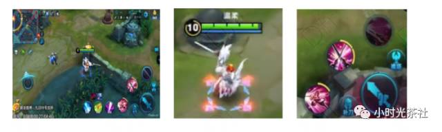
When designing classification features, it is necessary for the features to be as clear as possible, with significant differences between different categories.
3.2 Collecting Data
Collecting and labeling data is a tedious but crucial task; the same model may perform very differently under different training data. Here, we downloaded approximately 15 minutes of video for different heroes from YouTube and used the following ffmpeg command to capture images of the skill key area and compress their size.
ffmpeg -i videos/1/test.mp4 -r 1 -vf "crop=380:340:885:352,scale=224:224" images/1/test_%4d.pngThe dataset image folder is shown in the figure below. It is necessary to manually filter out noise images that do not contain skill keys and place them in the 0 folder. The 0 folder serves as the background classification, corresponding to the classification of heroes that cannot be recognized.
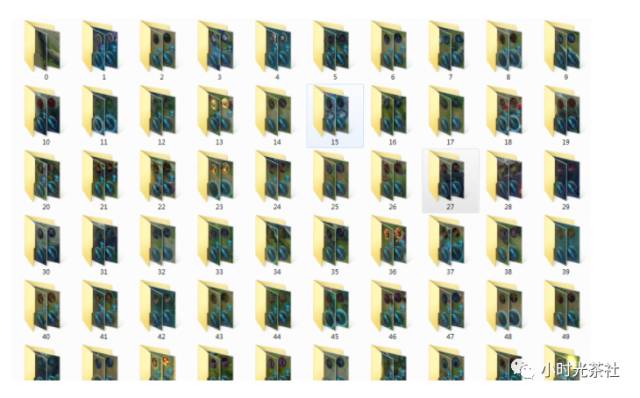
Each category contains approximately 1000-2000 images. The larger the dataset, the better, and it should cover as many scenarios as possible to increase the model’s generalization ability.
3.3 Processing Data
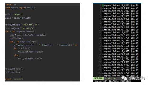
After generating the dataset, it needs to be converted into a format that Caffe can recognize. First, use the Python code on the left side of the figure below to generate the images contained in the training and testing sets, resulting in the file shown on the right side of the figure, which includes image paths and classifications. The testing set consists of one-fifth of all images.
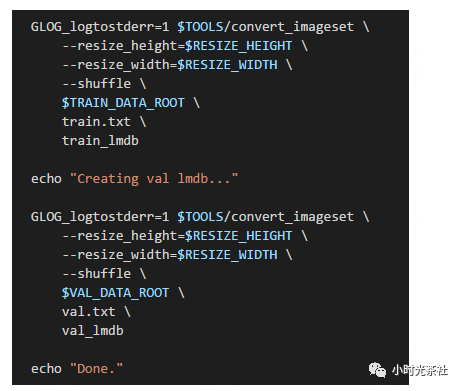
Next, convert the images to LMDB format data; Caffe provides tools to assist us in the conversion. The processing script is shown in the figure below.
3.4 Selecting a Model
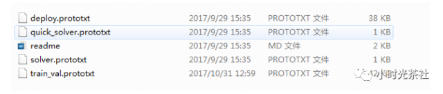
The six models introduced above are commonly used image classification models; here we choose GoogLeNet as the model network. In the models folder of the Caffe project, these network models can be found. Check the caffe/models/bvlc_googlenet folder, which contains the following files:
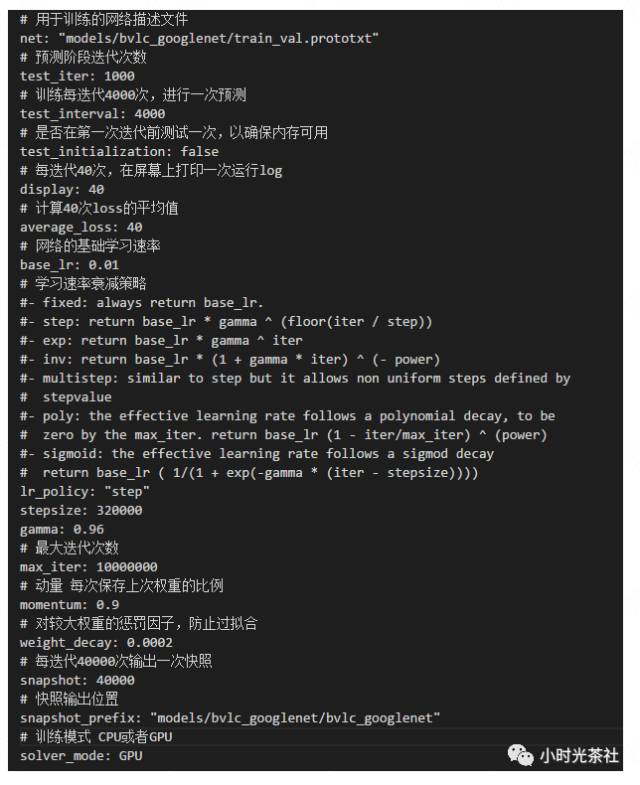
3.4.1 solver.prototxt
The solver.prototxt file defines the parameters used for training the model, with specific meanings shown in the figure below:
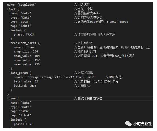
3.4.2 train_val.prototxt
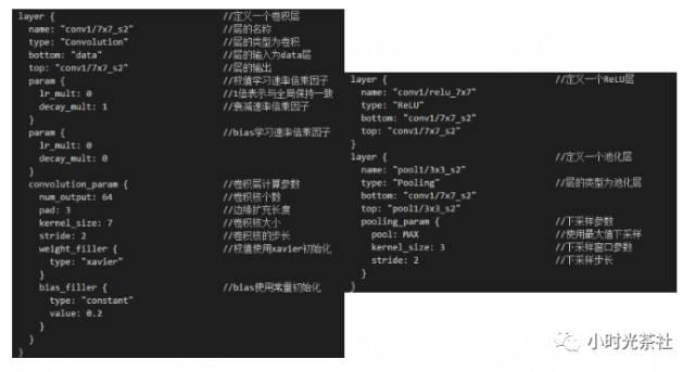
train_val.prototxt defines the specific structure of the GoogLeNet network. There are many network files; here we introduce the structure of independent network layers. First is the data layer, with parameters as shown in the figure below:
The structures of the convolutional layer, ReLU layer, and pooling layer are shown in the figure below:
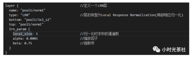
The structure of the LRN layer is shown in the figure below:
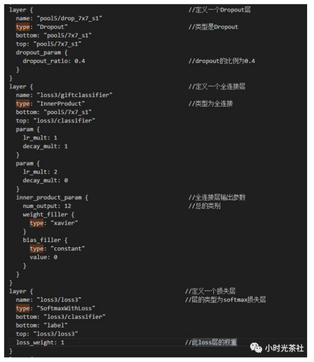
The structure of the Dropout layer and fully connected layer is shown in the figure below:
3.4.3 deploy.prototxt
The deploy file is the network structure used during deployment, most of its content is similar to the train_val.prototxt file, with some testing layers removed.
3.5 Training the Model
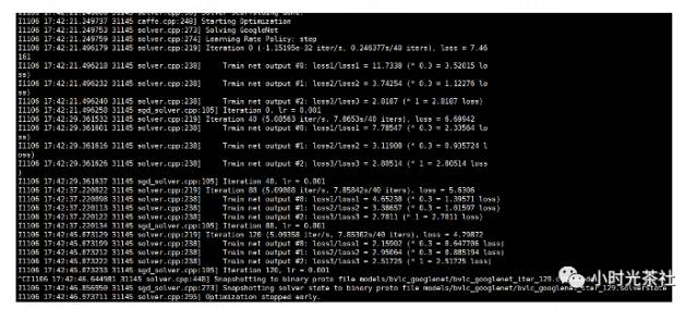
Once the data and model are prepared, we can start training the model. Here, we call the following code to begin training:
caffe train -solver solver.prototxtYou can add the -snapshot parameter to continue training from the last model. The training log is shown in the figure below:
When the model converges, or the accuracy reaches our requirements, training can be stopped.
3.6 Pruning the Model
GoogLeNet is a relatively large network, and we can prune the network according to our needs. The LRN layer in GoogLeNet has little impact and can be removed, or some convolutional layers can be deleted to reduce the number of layers in the network.
3.7 Fine-tuning
When our dataset is relatively small, training the complete network parameters can easily lead to overfitting. In this case, we can address this issue by only training certain layers of the network. First, modify the names of the fully connected layers in train_val.prototxt, i.e., loss1/classifier, loss2/classifier, loss3/classifier, and their output classification counts, which default to 1000, need to be changed to our total number of categories. This way, when we load the pre-trained model, the parameters of these three layers will be reinitialized. Then set the lr_mult of all other layers to 0, so that the parameters of other layers will not change, using pre-trained parameters. Download bvlc_googlenet.caffemodel, which contains parameters trained by Google on ImageNet. Then call caffe train -solver solver.prototxt -weights bvlc_googlenet.caffemodel to train.
Tips
Local Minima Problem: A feasible trick is to reduce the batch size during the initial phase.
Loss Explosion: Reduce the learning rate.
Loss Never Converges: Suspect that there may be issues with the dataset or labels.
Overfitting: Strategies such as data augmentation, regularization, dropout, batch normalization, and early stopping can be employed.
Weight Initialization: Generally, use Xavier or Gaussian initialization.
Fine-tune: Use GoogLeNet or VGG; fine-tuning can be done on existing models.
Reference Documents:
1. This article is mainly organized from CS231n course notes, with the Chinese translation link https://zhuanlan.zhihu.com/p/21930884. The Chinese open course link is http://study.163.com/course/introduction/1003223001.htm. Strongly recommended for everyone to take a look.
2. Yoshua Bengio’s “Deep Learning Book” is highly recommended and definitely worth reading.
3. Zhou Zhihua’s “Machine Learning” is suitable for beginners in machine learning.
4. “TensorFlow Practical Implementation” is a good resource for TensorFlow practice.
5. Stanford University’s deep learning tutorial: http://ufldl.stanford.edu/wiki/index.php/UFLDL%E6%95%99%E7%A8%8B.
Author: Gao Chengcai, Android development engineer at Tencent, mainly responsible for the development and technical optimization of the Penguin Esports streaming SDK and the Penguin Esports APP.
Source: Hourglass Tea House