Intelligent Prediction of Loose Circles in Deep Tunnels Based on Improved XGBoost Algorithm

Introduction

Since the beginning of the 21st century, with the rapid development of the social economy, the demand for resources has continued to increase. However, shallow mineral resources are increasingly depleted, forcing mining work to shift underground. After blasting and excavating deep tunnels, the surrounding rock inevitably produces a loose circle due to the coupling effect of explosive shock and dynamic unloading of in-situ stress, which in turn affects the stability of the structure. Therefore, it is very important to predict the thickness of the loose circle in advance.

The XGBoost algorithm is currently a mainstream machine learning algorithm, known for its high performance and scalability. This algorithm integrates regularization techniques internally and supports cross-validation, thereby improving the model’s generalization ability and reducing the risk of overfitting. Senior Engineer Fan Xingyu and his team from the Nuclear Industry Well Tunnel Construction Group Co., Ltd. first constructed a loose circle thickness prediction model based on the XGBoost model and optimized the model using GA, GWO, PSO, and SSA to further improve the prediction accuracy and reliability of the loose circle thickness. Secondly, 300 sets of effective loose circle data samples were obtained based on underground mine blasting excavation projects. A comparative analysis of four hybrid models and four benchmark models was conducted based on R2, RMSE, MAE, and MAPE model performance indicators, and sensitivity analysis of the parameters affecting the loose circle was performed using the XGBoost algorithm. Finally, the PSO-XGBoost model was used for predicting the loose circle of the surrounding rock in the transportation tunnel of the Wushan Copper Mine, thus verifying the reliability of the model in practical engineering.

1 Loose Circle Data

The loose circle is often generated after the excavation of underground tunnels is completed, primarily due to the combined effects of explosive shock loads and the stress field re-distributed after the excavation of the rock mass (Figure 1). In-situ tests of the loose circle were conducted using the SETPLT-02 acoustic detector at Linglong Gold Mine, Fankou Lead-Zinc Mine, and Wushan Copper Mine. Geological surveys and core sampling were conducted at the test sites, followed by a series of rock mechanics tests. The geographical location of the test mines and the on-site testing process are shown in Figure 2. Fankou Lead-Zinc Mine is located in Renhua County, Shaoguan City, Guangdong Province, and is a large lead-zinc production base in China. The loose circle testing point is located in the -680 m return air tunnel, where the horizontal stress is relatively high. The surrounding rock of the tunnel is medium-strength calcareous sandstone, and significant deformation and damage were observed after blasting excavation.

Intelligent Prediction of Loose Circles in Deep Tunnels Based on Improved XGBoost Algorithm

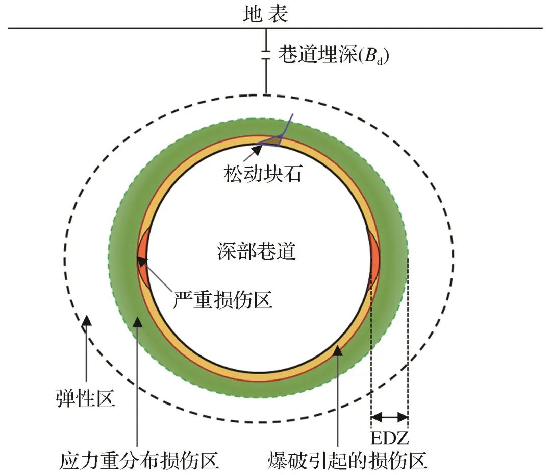
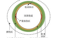
Figure 1 Schematic diagram of EDZ around deep tunnelsFig.1 Schematic diagram of EDZ around deep tunnels

Intelligent Prediction of Loose Circles in Deep Tunnels Based on Improved XGBoost Algorithm

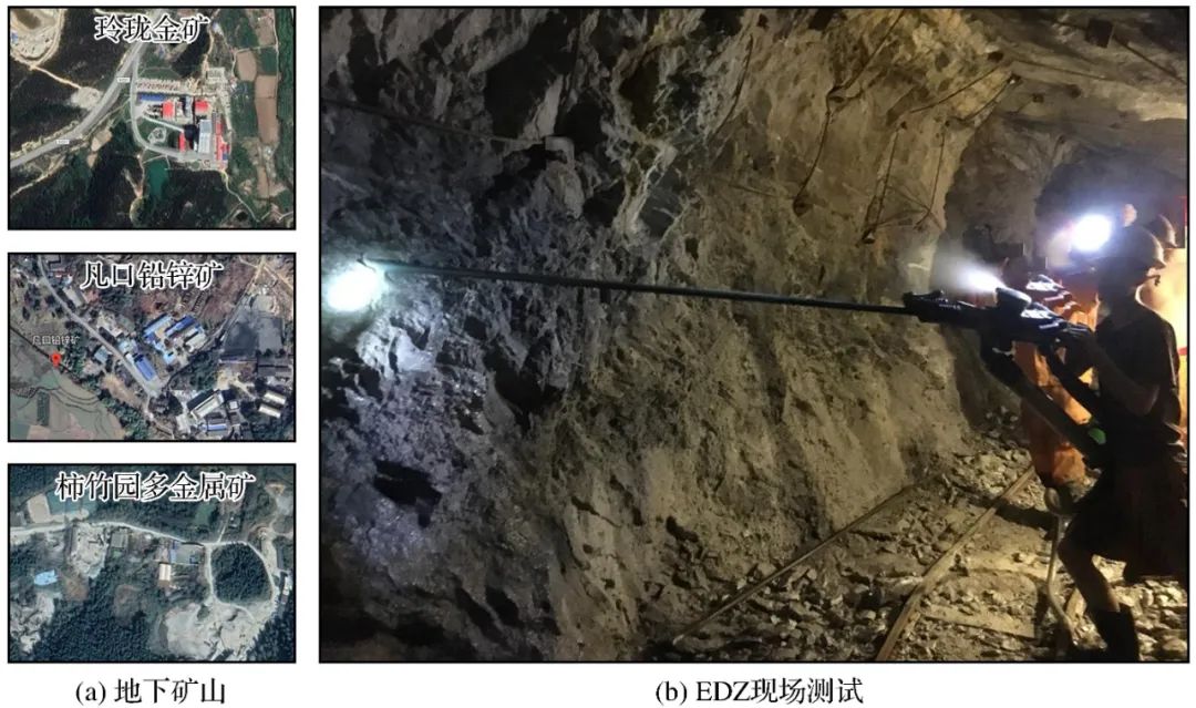
Figure 2 Underground mines conducting EDZ measurementsFig.2 Underground mines conducting EDZ measurements

Based on existing studies, the intelligent prediction based on the improved XGBoost model includes eight influencing factors of loose circle thickness, including geological strength index, uniaxial compressive strength of the rock mass, vertical principal stress, and charge coefficient, with the output parameter being the loose circle thickness. The influencing parameters and thickness data of the loose circle are shown in Table 1.

Table 1 Input and output parameters of EDZTable 1 Input and output parameters of EDZ

Intelligent Prediction of Loose Circles in Deep Tunnels Based on Improved XGBoost Algorithm
To visualize the data analysis, the eight input parameters and one output parameter were plotted in a violin form, as shown in Figure 3. In this sample data, the loose circle thickness is concentrated between 30~60 cm, and the overall distribution is relatively uniform. The GSI value violin plot is relatively wide, indicating that the parameter values are evenly distributed across the entire range. The violin plots of other input parameters are also relatively wide, indicating that the data distribution is also very uniform and highly reliable. It should be noted that the frequency is relatively low when the tunnel lateral pressure coefficient is less than 0.5, while it is mainly concentrated around 1.5.

Intelligent Prediction of Loose Circles in Deep Tunnels Based on Improved XGBoost Algorithm

Figure 3 Distribution of EDZ input and output parametersFig.3 Distribution of EDZ input and output parameters2 XGBoost and Optimization Algorithms

2.1 XGBoost Algorithm

XGBoost was initially proposed by Chen et al. (2016) and is a highly scalable machine learning system developed from the concept of gradient boosting decision trees (GBDT). Compared with GBDT, the XGBoost model shows the following advantages: (1) it penalizes the complexity of the model to avoid overfitting; (2) it can process massive data in parallel at high computational speed; (3) it allows users to define the objective function as long as it is twice differentiable; (4) it effectively handles datasets involving missing values. Therefore, the XGBoost algorithm has been widely applied in many fields with excellent performance.
The computational process of the XGBoost algorithm is shown in Figure 4. The algorithm complexity in XGBoost is optimized as part of the objective function, whose expression is as follows:
Intelligent Prediction of Loose Circles in Deep Tunnels Based on Improved XGBoost Algorithm (1)
Where: l is the loss function; Ω is the regularization term function.

Intelligent Prediction of Loose Circles in Deep Tunnels Based on Improved XGBoost Algorithm

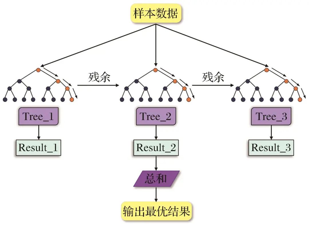
Figure 4 Schematic diagram of intelligent prediction structure by XGBoost algorithmFig.4 Schematic diagram of intelligent prediction structure by XGBoost algorithm

Due to Intelligent Prediction of Loose Circles in Deep Tunnels Based on Improved XGBoost Algorithm
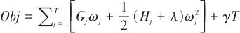
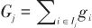
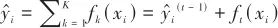
, the objective function at the tth iteration can be described by a more specific mathematical model, expressed as
Intelligent Prediction of Loose Circles in Deep Tunnels Based on Improved XGBoost Algorithm (2)
Then, the objective function is optimized through three steps, and the final form of the objective function is as follows:
Intelligent Prediction of Loose Circles in Deep Tunnels Based on Improved XGBoost Algorithm (3)
Where: Intelligent Prediction of Loose Circles in Deep Tunnels Based on Improved XGBoost Algorithm; Intelligent Prediction of Loose Circles in Deep Tunnels Based on Improved XGBoost Algorithm. In summary, the XGBoost algorithm transforms the search for the optimal target value into a problem of finding the minimum by establishing a quadratic equation of the variables.

2.2 GA Algorithm

GA (Genetic Algorithm) was first proposed and developed by Holland (1992). The working principle of this algorithm is to maintain a population of candidate solutions, called individuals or chromosomes, representing potential solutions to the problem at hand. The genetic algorithm mimics the process of natural selection, evolving this population over several generations, consisting of five key steps: initialization, evaluation, selection, reproduction, and replacement (Yang, 2021), with the process of obtaining the optimal value shown in Figure 5.

Intelligent Prediction of Loose Circles in Deep Tunnels Based on Improved XGBoost Algorithm

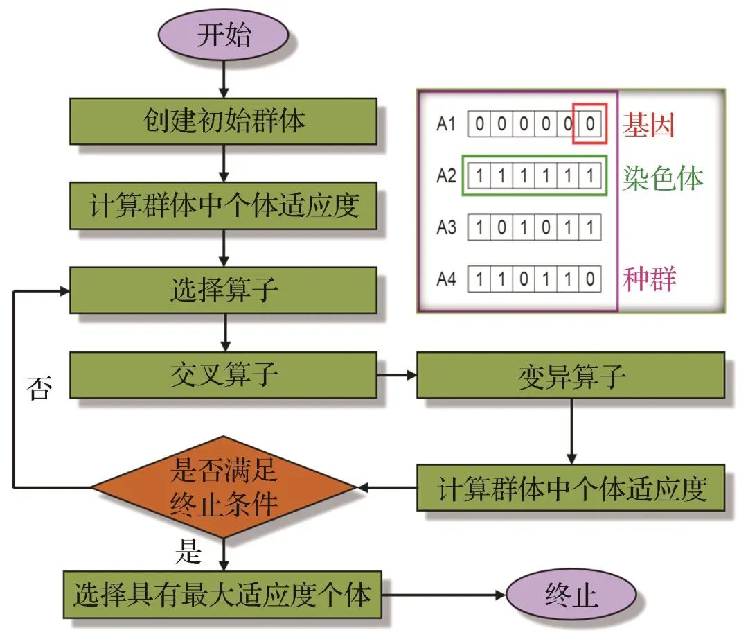
Figure 5 Flow chart of GA algorithmFig.5 Flow chart of GA algorithm

Through several generations, the genetic algorithm tends to improve the overall fitness of the population and converge towards better solutions to the problem. By exploring different gene combinations and gradually refining them, this algorithm can find the best or near-optimal solutions for a wide range of complex problems.

2.3 GWO Algorithm

GWO (Grey Wolf Optimizer) is a novel algorithm based on swarm intelligence proposed by Mirjalili et al. (2014). GWO forms a strict hierarchical structure inspired by the hunting and social behavior of wolves, with different wolves playing different roles within the grey wolf pack. Each wolf is governed by a harsh social order. The GWO algorithm process is shown in Figure 6.

Intelligent Prediction of Loose Circles in Deep Tunnels Based on Improved XGBoost Algorithm

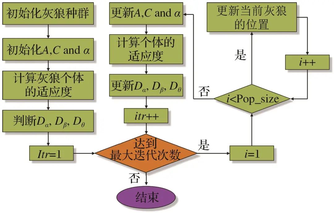
Figure 6 Flow chart of GWO algorithmFig.6 Flow chart of GWO algorithm

2.4 PSO Algorithm

PSO (Particle Swarm Optimization) is a powerful method among many evolutionary search methods used to solve optimization problems, implemented by simulating fish schools and bird flocks (Kennedy, 1995). The PSO algorithm process is shown in Figure 7, where the bird flock represents a group of particles, and the food source represents a functional objective. By sharing and transmitting distance information between the bird flock and the food source, the position of the food source can be determined by the bird flock. This cooperation allows the entire bird flock to select the best information regarding the food source location and ultimately converge around the food. During the computation, some important parameters in the PSO algorithm are updated, which can determine new positions and velocities.

Intelligent Prediction of Loose Circles in Deep Tunnels Based on Improved XGBoost Algorithm

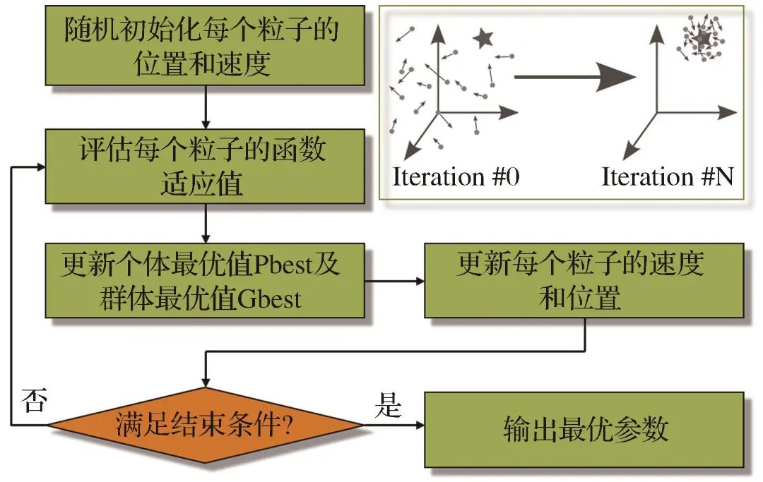
Figure 7 Flow chart of PSO algorithmFig.7 Flow chart of PSO algorithm
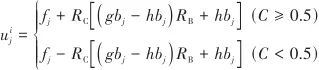
2.5 SSA Algorithm

Similar to the above two algorithms, SSA (Salp Swarm Algorithm) belongs to a group of optimization algorithms based on swarm intelligence (Cortés-Caicedo et al., 2022), inspired by the hunting and navigation behavior of salps. In the SSA algorithm, there are three main steps to optimize hyperparameters: initialization of the salp swarm, updating the leaders, and updating the followers. During the initialization process, the number and position of the salp swarm need to be defined. In addition, the best food source (fitness function) must be determined based on user requirements. In the next step, the optimization process begins within the search domain, which can be represented by a matrix named Si:
Intelligent Prediction of Loose Circles in Deep Tunnels Based on Improved XGBoost Algorithm (4)
In this search space, the leader will act first, providing guidance to the followers. The updating equation for the leader salp’s position is
Intelligent Prediction of Loose Circles in Deep Tunnels Based on Improved XGBoost Algorithm (5)
Where: gbj and hbj are the search upper and lower bounds in the j dimension; fj is the food location in the j dimension; RB and RC are two random parameters with values in [0, 1]. The parameter RB determines the length of the salp’s movement and can control the direction of movement. The parameter RC plays an important role in controlling exploration and exploitation.
Repeat the above steps until optimization reaches the stopping criteria. The optimization process of the SSA algorithm is shown in Figure 8.

Intelligent Prediction of Loose Circles in Deep Tunnels Based on Improved XGBoost Algorithm

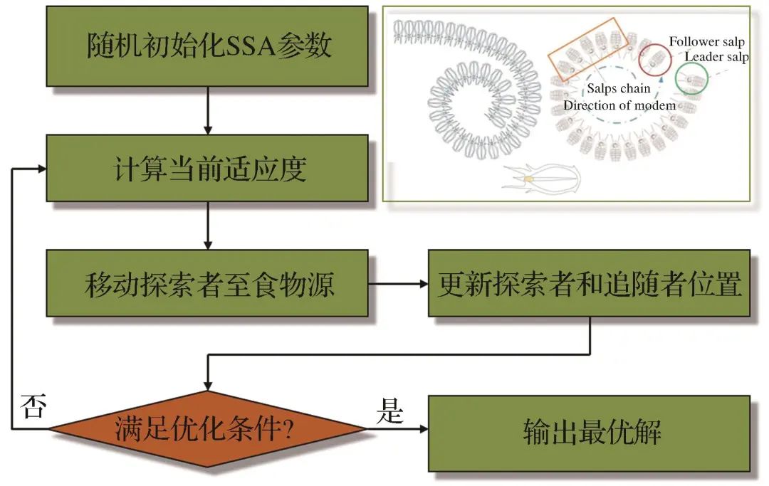
Figure 8 Flow chart of SSA algorithmFig.8 Flow chart of SSA algorithm

2.6 Hybrid Loose Circle Prediction Model Based on XGBoost

Four optimization algorithms were selected to adjust the hyperparameters of XGBoost to construct an intelligent prediction hybrid model for loose circle thickness, namely GA-XGBoost, GWO-XGBoost, PSO-XGBoost, and SSA-XGBoost. Although the optimization ideas of the four algorithms are quite different, the overall architecture of the corresponding four models is very similar and can be summarized in the following five steps: (1) experimental data preprocessing; (2) model parameter initialization; (3) population initialization; (4) iterative loop; (5) output optimal solution. Taking the GWO-XGBoost model as an example, the loose circle thickness prediction process is shown in Figure 9.

Intelligent Prediction of Loose Circles in Deep Tunnels Based on Improved XGBoost Algorithm

Figure 9 GWO-XGBoost model processFig.9 Flow chart of the GWO-XGBoost model

2.7 Model Performance Evaluation Indicators

The constructed prediction model is evaluated using performance indicators (PI), including Root Mean Square Error (RMSE), Mean Absolute Error (MAE), Mean Absolute Percentage Error (MAPE), and Standard Deviation (R2). Assuming RMSE = 0, MAE = 0, MAPE = 0, R2 = 1, the prediction model is deemed highly reliable. The expressions for the performance evaluation indicators of the four models are as follows:
Intelligent Prediction of Loose Circles in Deep Tunnels Based on Improved XGBoost Algorithm (6)
Intelligent Prediction of Loose Circles in Deep Tunnels Based on Improved XGBoost Algorithm (7)
Intelligent Prediction of Loose Circles in Deep Tunnels Based on Improved XGBoost Algorithm (8)
Intelligent Prediction of Loose Circles in Deep Tunnels Based on Improved XGBoost Algorithm (9)
Where: yi, Intelligent Prediction of Loose Circles in Deep Tunnels Based on Improved XGBoost Algorithm, and Intelligent Prediction of Loose Circles in Deep Tunnels Based on Improved XGBoost Algorithm are the true value, predicted value, and mean value of the true value of the ith sample, respectively; n is the sample size.
3 Results and Analysis
To construct a loose circle thickness prediction model based on XGBoost for deep tunnel blasting, four meta-heuristic algorithms were used to optimize XGBoost. Eight influencing factors such as geological conditions, blasting parameters, and excavation characteristics were used as inputs, with the loose circle thickness as the output. Among them, the number of swarms and the number of iterations play a key role in optimization performance. Therefore, a comparison and analysis of the Mean Square Error (MSE) of the hybrid model under different swarm sizes was conducted.

3.1 GWO-XGBoost Model

Generally, as the number of iterations increases, the optimization performance tends to stabilize, but the computation time also increases. To assess the optimization performance, the MSE value was analyzed. During the test process, the number of iterations for stable prediction performance was set to 500, and the swarm sizes (number of particles) of 60, 70, 80, 90, and 100 were tested to select the best optimal parameters. As shown in Figure 10, the variation process of each swarm size (number of particles) is different. As the number of iterations increases, the MSE value continues to decrease. Each model achieved the lowest MSE value upon reaching the optimization endpoint. From Figure 10, it can be seen that when the swarm size (number of particles) is 100, its optimal MSE value is greater than that of other swarm sizes (number of particles), and the optimal value corresponds to a much larger number of iterations than that of other swarm sizes (number of particles), indicating that the model is inefficient and unstable when the swarm size (number of particles) is 100. In contrast, when the swarm size (number of particles) is 90, the MSE value reaches a stable value at the minimum number of iterations (121), which is smaller than the MSE values of other swarm sizes, so it is considered that the GWO-XGBoost model has the best prediction performance when the swarm size (number of particles) is 90.

Intelligent Prediction of Loose Circles in Deep Tunnels Based on Improved XGBoost Algorithm

Figure 10 Variations of MSE value with iteration number of GWO-XGBoost model under different swarm sizesFig.10 Variations of MSE value with iteration number of GWO-XGBoost model under different swarm sizes

To further verify the prediction performance of the GWO-XGBoost model under different swarm sizes, MAW, MAPE, RMSE, and R2 in the training and testing sets were calculated, and the results are shown in Table 2. From Table 2, it can be seen that when the number of particles is 90, the GWO-XGBoost model achieves the best prediction performance, with MAW, MAPE, RMSE, and R2 in the training set being 6.812, 6.943, 9.522, and 0.9073, respectively. The number of particles with good predictive performance is 60, with a correlation coefficient above 0.9. When the number of particles is 100, the prediction performance of the GWO-XGBoost model is the worst, which is consistent with the conclusion in Figure 10, where MAW, MAPE, RMSE, and R2 in the training set are 8.212, 8.994, 11.705, and 0.8723, respectively. Therefore, it is concluded that when the number of particles is 90, the GWO-XGBoost model has the best fitting ability and optimal prediction performance in both the training and testing sets.

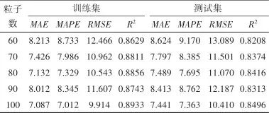
Table 2 Performance of GWO-XGBoost model under different swarm sizesTable 2 Performance of GWO-XGBoost model under different swarm sizes

Intelligent Prediction of Loose Circles in Deep Tunnels Based on Improved XGBoost Algorithm

3.2 GA-XGBoost Model

The GA algorithm can enhance the parameter selection of the XGBoost model. Before using GA-XGBoost for predicting loose circle thickness, the most effective GA parameters were selected. Similar to the construction of the GWO-XGBoost model, this section will discuss the impact of the number of iterations and swarm size on prediction performance. The swarm sizes (number of particles) were set to 60, 70, 80, 90, and 100, and the corresponding MSE values and iteration curves are shown in Figure 11.

Intelligent Prediction of Loose Circles in Deep Tunnels Based on Improved XGBoost Algorithm

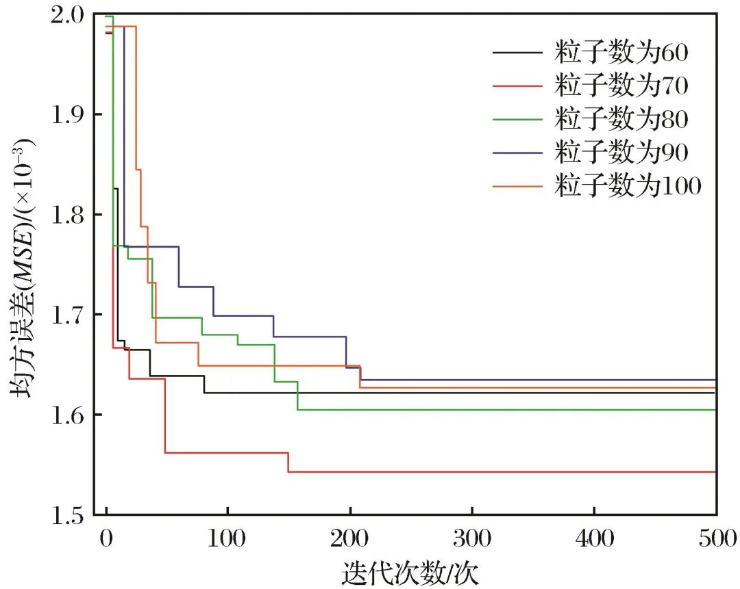
Figure 11 Variations of MSE value with iteration number of GA-XGBoost model under different swarm sizesFig.11 Variations of MSE value with iteration number of GA-XGBoost model under different swarm sizes

From Figure 11, it can be seen that when the number of particles is 70, the GA-XGBoost model achieves the minimum MSE value, and the number of iterations corresponding to the stable MSE value is also relatively small. As shown in Table 3, when the number of particles is 70, the training set values are MAW=7.483, MAPE=7.201, RMSE=10.423, and R2=0.8734, while the testing set values are MAW=8.802, MAPE=7.777, RMSE=11.257, and R2=0.8384. However, when the number of particles is 90, the overall prediction performance of the GA-XGBoost model is the worst, as the MSE value corresponding to the convergence of the fitness curve is the largest, and the number of iterations is also the largest at 208, indicating that the model’s stability and reliability are at their worst under this swarm size. When the number of particles is 90, the training set values are MAW=8.312, MAPE=8.834, RMSE=12.795, and R2=0.8432, while the testing set values are MAW=8.977, MAPE=9.433, RMSE=13.819, and R2=0.8098.

Table 3 Performance of GA-XGBoost model under different swarm sizesTable 3 Performance of GA-XGBoost model under different swarm sizes

Intelligent Prediction of Loose Circles in Deep Tunnels Based on Improved XGBoost Algorithm

3.3 PSO-XGBoost Model

Figure 12 shows the variation of the MSE values with the number of iterations for the PSO-XGBoost model under different swarm sizes (number of particles). From Figure 12, it can be seen that regardless of whether the swarm size is small (60 or 70 particles) or large (100 particles), the MSE values rapidly decrease in the initial stage and then gradually stabilize. However, it is evident that the converged MSE values and corresponding iteration counts differ for different swarm sizes. Specifically, when the number of particles is 60 and 70, the MSE values are the smallest, with only a minimal difference between them. However, the convergence speed of the model when the number of particles is 60 is faster than when it is 70. When the number of particles is 90, the MSE value is the largest, indicating the worst stability of the model. When the number of particles is 100, the convergence MSE value corresponds to the largest number of iterations, indicating the slowest convergence speed and poor performance of the model.

Intelligent Prediction of Loose Circles in Deep Tunnels Based on Improved XGBoost Algorithm

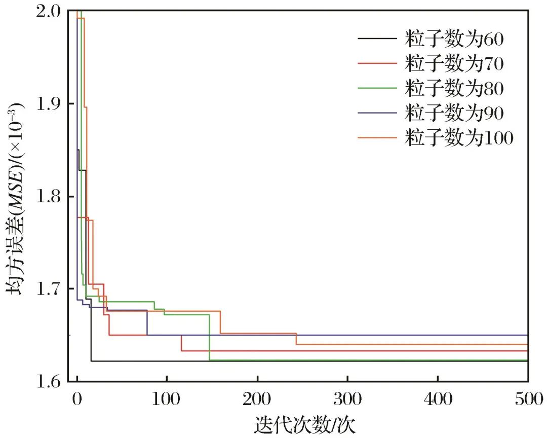
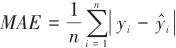
Figure 12 Variations of MSE value with Iteration number of PSO-XGBoost model under different swarm sizesFig.12 Variations of MSE value with Iteration number of PSO-XGBoost model under different swarm sizes

To comprehensively compare the performance of the models in predicting loose circle thickness under different swarm sizes, the performance indicator values in the training and testing sets were calculated, and the results are listed in Table 4. From Table 4, it can be seen that when the swarm size (number of particles) is 60, the PSO-XGBoost model exhibits the best prediction performance, with training set values of MAW=5.231, MAPE=5.513, RMSE=7.143, and R2=0.9244, while the testing set values are MAW=5.543, MAPE=5.844, RMSE=77.752, and R2=0.8787. All indicators are better than when the number of particles is 70. When the number of particles is 90, both the correlation coefficient in the training and testing sets are the smallest, and MAE, MAPE, and RMSE are the largest, indicating the worst prediction performance of the model under this swarm size.

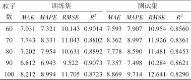
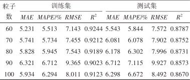
Table 4 Performance of PSO-XGBoost model under different swarm sizesTable 4 Performance of PSO-XGBoost model under different swarm sizes

Intelligent Prediction of Loose Circles in Deep Tunnels Based on Improved XGBoost Algorithm

3.4 SSA-XGBoost Model

As a novel swarm intelligence algorithm, SSA has shown its superiority and feasibility in various optimization problems. SSA is easy to implement and adjust. For ease of comparison, the same hyperparameter values were also used in the SSA-based model. Figure 13 shows the optimization process of the SSA-XGBoost model under different swarm sizes. From Figure 13, it can be seen that the SSA-XGBoost model gradually stabilizes with the increase in the number of iterations under different swarm sizes, indicating that the model approaches the optimal solution during the iteration process. However, the sizes of the converged mean square error values and the convergence speeds differ. When the number of particles is 100, the model converges with the smallest MSE value and the fastest convergence speed, corresponding to 95 iterations. The swarm size (number of particles) with the best convergence performance is 80. It is evident that when the number of particles is 60, although the model converges quickly, the MSE value is the largest, indicating the poor stability of the model at this swarm size.

Intelligent Prediction of Loose Circles in Deep Tunnels Based on Improved XGBoost Algorithm

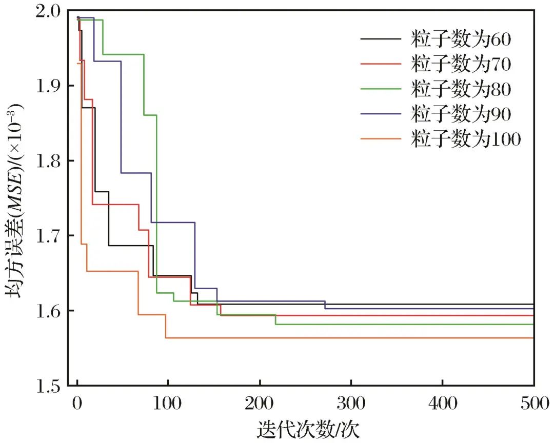
Figure 13 Variations of MSE value with iteration number of SSA-XGBoost model under different swarm sizesFig.13 Variations of MSE value with iteration number of SSA-XGBoost model under different swarm sizes

Table 5 shows the evaluation index values of the models under different swarm sizes. When the number of particles is 100, both in the training and testing sets, the correlation coefficient is greater than that of other swarm sizes, while MAE, MAPE, and RMSE are smaller, indicating that this model has the best overall prediction performance. At the same time, the data in Table 5 further confirm that the performance of the SSA-XGBoost model is the worst when the number of particles is 60, with MAW=8.213, MAPE=8.733, RMSE=12.46, R2=0.8629 in the training set, and the evaluation indicators in the testing set are MAW=8.624, MAPE=9.170, RMSE=13.089, R2=0.8208.

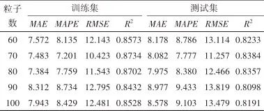
Table 5 Performance of SSA-XGBoost model under different swarm sizesTable 5 Performance of SSA-XGBoost model under different swarm sizes

Intelligent Prediction of Loose Circles in Deep Tunnels Based on Improved XGBoost Algorithm

3.5 Model Comparison Analysis

Based on the above discussion, the GWO-XGBoost model, GA-XGBoost model, PSO-XGBoost model, and SSA-XGBoost model exhibit the best prediction performance when the number of particles is 90, 70, 60, and 100, respectively. Therefore, these four models with the best performance under these swarm sizes were selected to predict 60 sets of test data, along with the unoptimized XGBoost model and three common models: SVM, RF, and LightGBM, for comparative analysis of the advantages and disadvantages of these eight models. Figure 14 shows the two-dimensional distribution and linear fitting of predicted values and actual values for various prediction models. As shown in Figure 14, the data points in the PSO-XGBoost model cluster near the linear fitting curve, with a 95% prediction bandwidth relatively narrower than that of other models. The data points of the other seven loose circle prediction models are more dispersed than those of the PSO-XGBoost model, especially for the LightGBM and SVM models, indicating that the PSO-XGBoost model has more accurate and stable prediction performance, making it the most suitable for predicting the thickness of loose circles in surrounding rock after blasting excavation of deep tunnels. Furthermore, comparing the hybrid models (GWO-XGBoost, GA-XGBoost, PSO-XGBoost, and SSA-XGBoost) with the benchmark models (XGBoost, SVM, RF, Light-GBM), it is evident that the optimized models have better prediction performance.

Intelligent Prediction of Loose Circles in Deep Tunnels Based on Improved XGBoost Algorithm

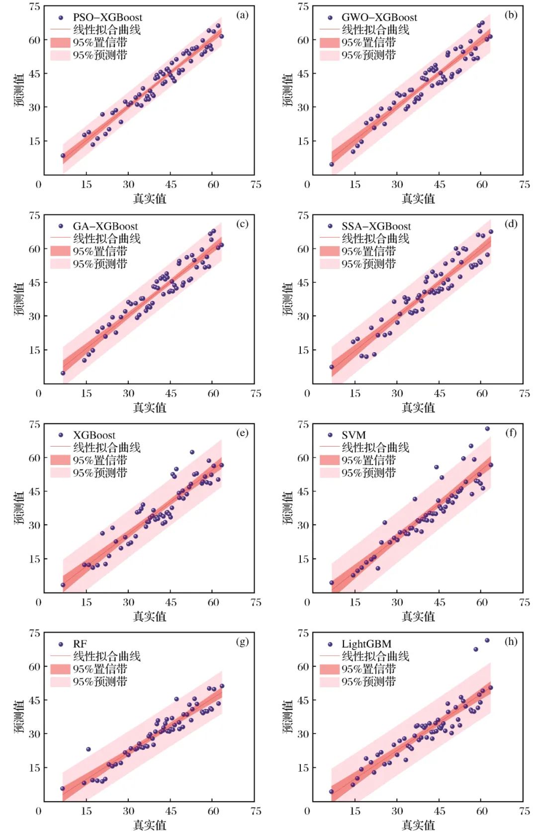
Figure 14 Comparison of predicted values and actual values of different modelsFig.14 Comparison of predicted values and actual values of different models

To further quantify the performance of the eight models, the four performance indicators (MAE, MAPE, RMSE, and R2) of the training and testing sets were plotted in a radar chart (Figure 15). Figure 15(a) shows the distribution of MAE values for different models. It is evident that the PSO-XGBoost model has the smallest MAE values in both the training and testing sets, followed by the GWO-XGBoost model. The LightGBM model has the largest MAE value, indicating that the PSO-XGBoost model has the best intelligent prediction performance for loose circle thickness, while the LightGBM model performs the worst. Figure 15(b) shows the MAPE values of each model, with distribution characteristics similar to those of the MAE values. The MAPE values for the PSO-XGBoost model in the training and testing sets are 5.513 and 5.844, respectively, followed by the GWO-XGBoost model, with MAPE values of 6.943 and 7.498 in the next training and testing sets. The benchmark models have significantly larger MAPE values than the optimized models, with the LightGBM model’s MAPE values being 11.310 and 12.215, further confirming the prediction performance of the PSO-XGBoost model. Figures 15(b) and 15(c) show the RMSE and R2 values of each model. For RMSE, the LightGBM and SVM models have the largest values, while the PSO-XGBoost and GWO-XGBoost models have the smallest values. For R2, the situation is exactly the opposite, with the PSO-XGBoost and GWO-XGBoost models having the highest correlation coefficients in the training set, 0.9244 and 0.9073, respectively, while the LightGBM and SVM models have correlation coefficients of 0.8243 and 0.8376 in the training set.

Intelligent Prediction of Loose Circles in Deep Tunnels Based on Improved XGBoost Algorithm

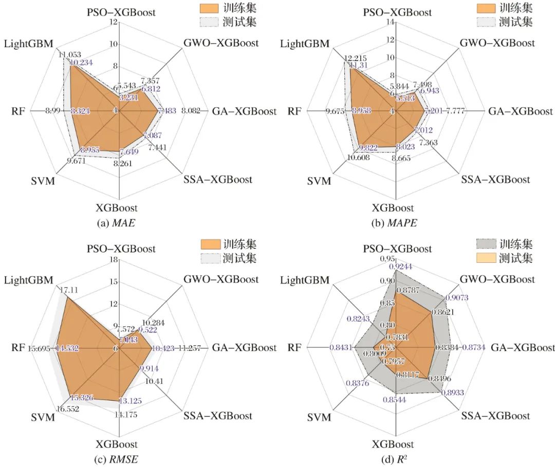
Figure 15 Comparison of performance evaluation indexes of different modelsFig.15 Comparison of performance evaluation indexes of different models

In summary, regardless of whether in the training set or testing set, the PSO-XGBoost model performs the best in prediction accuracy, generalization ability, and stability, followed by the GWO-XGBoost model. The benchmark model without hyperparameter adjustment exhibits poor stability and low prediction accuracy during the prediction process. Therefore, using the PSO-XGBoost and GWO-XGBoost models is reliable for the intelligent prediction of the thickness of loose circles in the surrounding rock during the excavation of underground tunnels using drilling and blasting methods.

3.6 Parameter Sensitivity Analysis

Parameter sensitivity analysis is a method to examine the stability of a system. In this study, after the network was created, sensitivity analysis was performed on the dataset. Sensitivity analysis checks the system’s tendencies and variations related to each model input. This is accomplished by changing the value of each input within the desired range. The general equation for sensitivity analysis is as follows:
Intelligent Prediction of Loose Circles in Deep Tunnels Based on Improved XGBoost Algorithm (10)
Where: Intelligent Prediction of Loose Circles in Deep Tunnels Based on Improved XGBoost Algorithm and k are dimensionless real numbers and are positive. Values greater than Intelligent Prediction of Loose Circles in Deep Tunnels Based on Improved XGBoost Algorithm indicate that the sensitivity of index p is higher relative to ak. By comparing different Intelligent Prediction of Loose Circles in Deep Tunnels Based on Improved XGBoost Algorithm values, the sensitivity strength of each input parameter can be obtained.
Using the XGBoost model, sensitivity detection was performed on all input parameters one by one, fixing other parameters during the detection of a certain parameter. The sensitivity values of the influencing factors of loose circle thickness were obtained and represented in histogram form, as shown in Figure 16. From Figure 16, it can be seen that the excavation diameter of deep tunnels (TD) has the greatest impact on the over-excavation thickness, with a sensitivity parameter of 0.73; followed by the geological strength index of the surrounding rock of the excavated tunnel, with a sensitivity parameter of 0.68. The study indicates that by adjusting the excavation size and enhancing the rock mass quality, the thickness of the loose circle after blasting excavation of deep tunnels can be effectively reduced. It is noteworthy that the vertical principal stress acting on the excavated tunnel also has a significant impact on loose circle thickness, with a sensitivity parameter of 0.56. For tunnels excavated using smooth blasting technology, the charge coefficient and spacing of the surrounding holes also have a certain strength of influence on loose circle thickness, so the distribution of the surrounding rock damage zone can be controlled by optimizing blasting parameters.

Intelligent Prediction of Loose Circles in Deep Tunnels Based on Improved XGBoost Algorithm

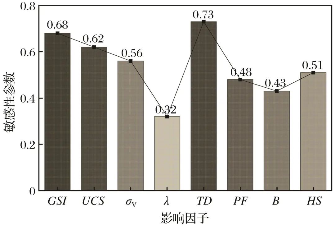
Figure 16 Sensitivity analysis of EDZ depth influencing factorsFig.16 Sensitivity analysis of EDZ depth influencing factors4 Engineering Verification

To further verify the reliability of the PSO-XGBoost loose circle thickness prediction model, this model was applied to the advance prediction of loose circles in the underground transportation tunnel of Wushan Copper Mine. Wushan Copper Mine belongs to Jiangxi Copper Co., Ltd., located in Baiyang Town, Xiri County, Jiujiang City, Jiangxi Province. The mining area includes two mineral belts, with significant differences in ore deposit conditions and a complex geological environment. The surrounding rock of the test tunnel is mainly white marble, accompanied by altered marble and sandstone along the entire excavation line. To minimize the damage to the surrounding rock during the blasting excavation process, smooth blasting technology was used for excavation. The tunnel excavation direction is parallel to the direction of the maximum horizontal principal stress, which can maximize the unloading of in-situ stress during excavation and prevent further damage to the rock mass. The design width of the tunnel is 3.4 m and the height is 3.0 m. Emulsified explosives were used on-site for rock fragmentation, and the smooth blasting parameters were adjusted according to the characteristics of the surrounding rock.
Six sections were selected along the tunnel line for the reliability verification of loose circle thickness prediction. The rock properties at different sections vary, obtained through indoor rock mechanics experiments and on-site joint fissure investigations. Before excavation, the PSO-XGBoost prediction model was used to predict the thickness of the loose circle based on rock parameters, blasting parameters, and the excavation diameter. After excavation was completed, on-site measurements of the loose circle at the test points were conducted, and the measurement results compared with the predicted values are listed in Table 6. From Table 6, it can be seen that the geological strength index (GSI) of the six test points is not equal, with the uniaxial compressive strength of intact rock samples ranging from 87.9 to 145.8 MPa. The charge coefficient for soft rock is smaller than that for hard rock, and the resistance line and hole spacing are larger, indicating that the selection of test points is representative. The loose circle thickness measurement results range from 13.43 to 35.12 cm, while the predicted values range from 13.87 to 38.01 cm, with the maximum prediction error being 9.5%, effectively controlled within 10%, indicating that the optimized PSO-XGBoost model performs well in engineering practice.

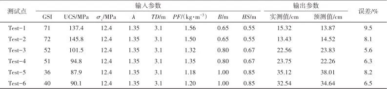
Table 6 Comparison of EDZ predicted value and measured valueTable 6 Comparison of EDZ predicted value and measured value

Intelligent Prediction of Loose Circles in Deep Tunnels Based on Improved XGBoost Algorithm
Therefore, it is possible to predict the thickness of the loose circle in advance before excavation in underground tunnels or chambers. On one hand, this allows for the optimization of blasting parameters based on the prediction results; on the other hand, it also facilitates the formulation of support schemes for surrounding rock after excavation.
5 Conclusion
(1) The swarm size and number of iterations have a significant impact on the performance of the prediction model. The GA-XGBoost, GWO-XGBoost, PSO-XGBoost, and SSA-XGBoost models achieve optimal prediction performance at swarm sizes (number of particles) of 90, 70, 60, and 100, respectively.
(2) PSO-XGBoost is the model with the best prediction performance among the four hybrid models, with correlation coefficients of 0.9244 and 0.8787 in the training and testing sets, respectively. The optimized four models have better performance in predicting loose circle thickness than the unoptimized XGBoost, RF, SVM, and LightGBM benchmark models, significantly improving prediction accuracy and stability after optimization using GA, GWO, PSO, and SSA algorithms.
(3) The results of parameter sensitivity analysis indicate that the relative importance of each input variable, from high to low, is the tunnel diameter, geological strength index of the surrounding rock, uniaxial compressive strength, vertical principal stress, spacing of smooth holes, charge coefficient, resistance line of smooth blasting, and lateral pressure coefficient. Therefore, it is essential to consider the influence of geological stress when predicting and analyzing the loose circle of surrounding rock in deep tunnels.
Intelligent Prediction of Loose Circles in Deep Tunnels Based on Improved XGBoost Algorithm

Chen T Q,Guestrin C,2016.XGBoost:A Scalable Tree Boosting System[C]//Proceedings of the 22nd ACM SIGKDD International Conference on Knowledge Discovery and Data Mining.San Francisco:Association for Computing Machinery:785-794.

Cortés-Caicedo B, Grisales-Noreña L F, Montoya O D,2022.Optimal selection of conductor sizes in three-phase asymmetric distribution networks considering optimal phase-balancing:An application of the salp swarm algorithm[J].Mathematics,10(18):3327.

Holland J H,1992.Adaptation in Natural and Artificial Systems:An Introductory Analysis with Applications to Biology,Control,and Artificial Intelligence[M].Cambridge:MIT Press.

Hong Z X,Tao M,Wu C Q,et al,2023.The spatial distribution of excavation damaged zone around underground roadways during blasting excavation[J].Bulletin of Engineering Geology and the Environment,82(4):155.

Hu Jun,Wang Kaikai,Xia Zhiguo,2014.Support vector machine(SVM)prediction of roadway surrounding rock loose circle thickness optimized by layered fish [J]. Metal Mine,43(11):31-34.

Kennedy J, Eberhart R,1995.Particle swarm optimization[C]//Proceedings of the IEEE International Conference on Neural Networks.Perth:IEEE.

Li S J,Feng X T,Li Z,et al,2012.Evolution of fractures in the excavation damaged zone of a deeply buried tunnel during TBM construction[J].International Journal of Rock Mechanics and Mining Sciences,55:125-138.

Liu Gang,Xiao Yongzhuo,Zhu Junfu,et al,2021.Overview on theoretical calculation method of broken rock zone[J].Journal of China Coal Society,46(1):46-56.

Liu Meng,Tang Hai,Ma Yujie,et al,2022.Measurement of loose zone of tunnel surrounding rock based on apparent resistivity method[J].Mineral Engineering Research,37(4):58-64.

Mirjalili S,Mirjalili S M,Lewis A,2014.Grey wolf optimizer[J]. Advances in Engineering Software,69:46-61.

Perras M A,Diederichs M S,2016.Predicting excavation damage zone depths in brittle rocks[J].Journal of Rock Mechanics and Geotechnical Engineering,8(1):60-74.

Qiao S,Cai Z,Xu P,et al,2021.Investigation on the scope and influence factors of surrounding rock loose circle of shallow tunnel under bias pressure:A case study[J]. Arabian Journal of Geosciences,14(15):1428.

Sun Q,Ma F,Guo J,et al,2021.Excavation-induced deformation and damage evolution of deep tunnels based on a realistic stress path[J].Computers and Geotechnics,129:103843.

Tang Dengzhi,Bai Genming,Chen Shuang,et al,2023.Research on influencing factors and prediction of rockburst in deep-buried tunnel[J].Sichuan Hydropowder,42(2):11-17.

Wang H W,Jiang Y,Xue S,et al,2015.Assessment of excavation damaged zone around roadways under dynamic pressure induced by an active mining process[J].International Journal of Rock Mechanics and Mining Sciences,77:265-277.

Wang R,Deng X,Meng Y,et al,2019.Case study of modified H-B strength criterion in discrimination of surrounding rock loose circle[J]. KSCE Journal of Civil Engineering,23(3):1395-1406.

Wang Xu,Li Xiaomeng,2023.Research on the present situation and development trend of loose zone test technology for roadway surrounding rock[J].Coal and Chemical Industry,46(1):4-7.

Wang Yong,Wu Aixiang,Yang Jun,et al,2023.Progress and prospective of the mining key technology for deep metal mines[J].Chinese Journal of Engineering,45(8):1281-1292.

Xie Heping,Gao Feng,Ju Yang,2015.Research and development of rock mechanics in deep ground engineering[J].Chinese Journal of Rock Mechanics and Engineering,34(11):2161-2178.

Xie Q,Peng K,2019.Space-time distribution laws of tunnel excavation damaged zones (EDZs) in deep mines and EDZ prediction modeling by random forest regression[J].Advances in Civil Engineering,(7):6505984.

Yang J H,Yao C,Jiang Q,et al,2017.2D numerical analysis of rock damage induced by dynamic in-situ stress redistribution and blast loading in underground blasting excavation[J].Tunnelling and Underground Space Technology,70:221-232.

Yang X S,2021.Genetic Algorithms[M].New York:Academic Press.

Yu Tao,Zhu Ningbo,Yao Zhigang,et al,2023.Stability analysis and control of tunnel excavation in deep buried horizontal stratum[J].Journal of Safety Science and Technology,19(4):93-99.

Zhou J,Li X B,2011.Evaluating the thickness of broken rock zone for deep roadways using nonlinear SVMs and multiple linear regression model[J].Procedia Engineering,26:972-981.

Zhu Zhijie,Zhang Hongwei,Chen Ying,2014.Prediction model of loosening zones around roadway based on MPSO-SVM [J].Computer Engineering and Applications,50(12):1-5.

胡军,王凯凯,夏治国,2014.分层鱼群优化支持向量机预测巷道围岩松动圈厚度[J].金属矿山,43(11):31-34.

刘刚,肖勇卓,朱俊福,等,2021.围岩松动圈理论计算方法的评述与展望[J].煤炭学报,46(1):46-56.

刘蒙,唐海,马谕杰,等,2022.基于视电阻率法测试技术的隧道围岩松动圈测定[J].矿业工程研究,37(4):58-64.

唐登志,白根铭,陈爽,等,2023.深埋隧道岩爆影响因素及其预测研究[J].四川水力发电,42(2):11-17.

王旭,李小萌,2023.巷道围岩松动圈测试技术现状及发展趋势研究[J].煤炭与化工,46(1):4-7.

王勇,吴爱祥,杨军,等,2023.深部金属矿开采关键理论技术进展与展望[J].工程科学学报,45(8):1281-1292.

谢和平,高峰,鞠杨,2015.深部岩体力学研究与探索[J].岩石力学与工程学报,34(11):2161-2178.

余涛,朱宁波,姚志刚,等,2023.深埋水平岩层隧道开挖稳定性分析及控制[J].中国安全生产科学技术,19(4):93-99.

朱志洁,张宏伟,陈蓥,2014.基于MPSO-SVM巷道围岩松动圈预测研究[J].计算机工程与应用,50(12):1-5.

Leave a Comment