Follow our WeChat public account “ML_NLP“
Set it as “Starred“, delivering heavy content as soon as possible!

Source | https://github.com/scutan90/DeepLearning-500-questions/blob/master/ch03_%E6%B7%B1%E5%BA%A6%E5%AD%A6%E4%B9%A0%E5%9F%BA%E7%A1%80/%E7%AC%AC%E4%B8%89%E7%AB%A0_%E6%B7%B1%E5%BA%A6%E5%AD%A6%E4%B9%A0%E5%9F%BA%E7%A1%80.md
https://zhuanlan.zhihu.com/p/105476748
This article is for interview experience sharing only and not for commercial use. If there is any infringement, please contact for deletion.
1. Why is it difficult to train deep neural networks?
1. Vanishing gradient. The vanishing gradient refers to the phenomenon where the gradient decreases as it moves backward through the hidden layers, indicating that the learning of the earlier layers is significantly slower than that of the later layers, leading to learning stagnation unless the gradient increases.
Causes of vanishing gradient: The size of the learning rate, the initialization of network parameters, the edge effects of activation functions, etc. In deep neural networks, the gradient computed by each neuron is passed to the previous layer, and the gradient received by shallower neurons is influenced by the gradients of all previous layers. If the computed gradient value is very small, as the number of layers increases, the gradient update information will decay exponentially, resulting in vanishing gradient.
2. Exploding gradient. In deep networks or structures like Recurrent Neural Networks (RNNs), the gradients can accumulate during the network update process, becoming very large, leading to significant updates in network weight values, causing instability in the network; in extreme cases, the weight values may overflow, becoming NaN, and can no longer be updated.
3. Degeneration of the weight matrix leads to a reduction in the effective degrees of freedom of the model.
The speed of learning degeneration in parameter space slows down, reducing the effective dimensionality of the model, and the available degrees of freedom in the network contribute unevenly to the gradient norm during learning. As the number of multiplied matrices (i.e., network depth) increases, the product of the matrices becomes increasingly degenerate. In nonlinear networks with hard saturation boundaries (e.g., ReLU networks), the degeneration process speeds up as depth increases.
2. What is the difference between deep learning and machine learning?
Traditional machine learning requires defining some handcrafted features to purposefully extract target information, relying heavily on task specificity and the expert experience of feature design. In contrast, deep learning can learn simple features from large datasets and gradually learn more complex abstract deep features without relying on manual feature engineering.
3. Why do we need nonlinear activation functions?
1. Activation functions can transform the current feature space into another space through certain linear mappings, learning and simulating other complex types of data such as images, videos, audio, and speech.
2. If the network consists entirely of linear components, then the linear combinations remain linear, which is no different from a single linear classifier. This would make it impossible to approximate arbitrary functions using nonlinearity.
3. Using nonlinear activation functions makes the network more powerful and increases its ability to learn complex things, complex structured data, and represent complex arbitrary function mappings between inputs and outputs. Nonlinear activation functions can generate nonlinear mappings between inputs and outputs.
4. What are the properties of activation functions?
2. Differentiability: This property is reflected when the optimization method is gradient-based;
3. Monotonicity: When the activation function is monotonic, a single-layer network can guarantee it is a convex function;
4. f(x)≈x: When the activation function satisfies this property, if the parameter initialization is a small random value, the training of the neural network will be efficient; if this property is not satisfied, detailed initial value settings are required;
5. Range of output values: When the output values of the activation function are finite, gradient-based optimization methods will be more stable, as the representation of features is significantly influenced by finite weights; when the output of the activation function is infinite, model training will be more efficient, but in this case, a smaller learning rate is generally needed.
5. How to choose activation functions?
-
If the output is binary (0, 1 values), then choose the sigmoid function for the output layer, and choose the ReLU function for all other units.
-
If uncertain which activation function to use in the hidden layers, the ReLU activation function is typically used. Sometimes, the tanh activation function is also used, but one advantage of ReLU is that when it is negative, the derivative equals 0.
-
Sigmoid activation function: It is rarely used except for binary classification problems in the output layer.
-
Tanh activation function: Tanh is very excellent and suitable for almost all situations.
-
If encountering dead neurons, we can use the Leaky ReLU function.
6. Advantages of ReLU activation function
1. The derivatives of sigmoid and tanh functions approach 0 in the positive and negative saturation regions, causing gradient dispersion, while the ReLU and Leaky ReLU functions are constant in the positive region and do not produce gradient dispersion.
2. In cases of large interval fluctuations, the derivatives or slopes of the ReLU activation function will be much greater than 0. In implementation, it is just an if-else statement, while the sigmoid function requires floating-point arithmetic, making the training of neural networks using ReLU activation function generally faster than using sigmoid or tanh activation functions.
3. It should be noted that when ReLU enters the negative half-space, the gradient is 0, and the neuron will not be trained, producing the so-called sparsity, while Leaky ReLU does not have this issue.
Sparse activation: From the signal perspective, this means that neurons selectively respond only to a small portion of input signals, intentionally filtering out a large number of signals, which can improve learning accuracy and better and faster extract sparse features. When x<0, ReLU is hard saturated, while when x>0, there is no saturation issue. ReLU can maintain the gradient without decay when x>0, thus alleviating the vanishing gradient problem.
7. Cross-entropy loss function and its derivation
There are two reasons to consider cross-entropy as a cost function.
First, it is non-negative, C > 0. It can be seen that all independent terms in the summation in the formula are negative because the domain of the logarithm function is (0, 1), and there is a negative sign before the summation, so the result is non-negative.
Second, if the actual output of the neuron is close to the target value for all training inputs x, then the cross-entropy will approach 0. The smaller the difference between the actual output and the target output, the lower the final value of the cross-entropy will be. (Here it is assumed that the output result is either 0 or 1, and the actual classification is similar.)
The cross-entropy cost function has a better property than the quadratic cost function, as it avoids the problem of decreasing learning speed.
The partial derivative of the cross-entropy function concerning weights:
After simplification, we obtain:
It can be seen that the learning speed is affected by the error in the output. Greater errors lead to faster learning speeds, particularly because this cost function avoids the slow learning caused by similar equations in the quadratic cost function. When we use cross-entropy, the error term is eliminated, so we no longer need to worry about it becoming very small. This cancellation is the special effect brought by cross-entropy.
8. Why does Tanh converge faster than Sigmoid?
As can be seen from the two formulas above, the vanishing gradient problem of tanh(x) is less severe than that of sigmoid, so Tanh converges faster than Sigmoid.
9. Why do we need Batch_Size?
The choice of batch determines the direction of descent.
If the dataset is relatively small, the full dataset can be used, with the benefits being:
-
The direction determined by the full dataset can better represent the sample population, thus more accurately pointing towards the direction of the extreme value.
-
Due to the significant differences in gradient values for different weights, selecting a global learning rate is challenging. Full Batch Learning can use Rprop based solely on gradient signs and specifically update each weight.
For larger datasets, if the full dataset is used, the disadvantages are:
-
As the dataset grows massively and memory limitations arise, loading all data at once becomes increasingly impractical.
-
Iterating using Rprop may lead to the sampling differences between each batch cancelling each other out, making it impossible to correct. This led to the later compromise solution of RMSProp.
10. Choosing the value of Batch_Size
If training with only one sample each time, i.e., Batch_Size = 1. The error surface of linear neurons in the mean squared error cost function is a paraboloid, with the cross-section being elliptical. For multi-layer neurons and nonlinear networks, locally it still approximates a paraboloid. At this point, each correction direction is adjusted based on the gradient direction of each sample, leading to difficulty in achieving convergence.
Since both Batch_Size for the full dataset and Batch_Size = 1 have their drawbacks, can a moderate Batch_Size value be chosen?
At this point, mini-batch gradient descent (Mini-batches Learning) can be employed. If the dataset is sufficiently ample, the gradient computed from using half (or even much less) of the data is almost identical to that computed using the entire dataset.
11. What are the benefits of increasing Batch_Size within a reasonable range?
-
Memory utilization improves, and the parallel efficiency of large matrix multiplication increases.
-
The number of iterations required to complete one epoch (the full dataset) decreases, further speeding up the processing of the same amount of data.
-
Within a certain range, generally speaking, the larger the Batch_Size, the more accurate the determined descent direction, leading to smaller training fluctuations.
12. What are the drawbacks of blindly increasing Batch_Size?
-
Memory utilization increases, but the memory capacity may not be able to hold it.
-
The number of iterations required to complete one epoch (the full dataset) decreases, but to achieve the same accuracy, the time taken increases significantly, resulting in slower parameter updates.
-
When Batch_Size increases to a certain extent, the determined descent direction no longer changes significantly.
13. Why normalize?
-
Avoid neuron saturation. When the activation of neurons approaches 0 or 1, saturation occurs, and in these regions, the gradient is almost 0, which can effectively “kill” the gradient during backpropagation.
-
Ensure that small values in the output data are not overwhelmed.
-
Accelerate convergence. There often exist outlier samples in the data, which can increase training time and may cause the network to fail to converge. To avoid this and facilitate subsequent data processing, normalizing the input signals can speed up network learning, making the mean of all samples’ input signals close to 0 or very small relative to their variance.
14. Why can normalization improve the speed of finding optimal solutions?
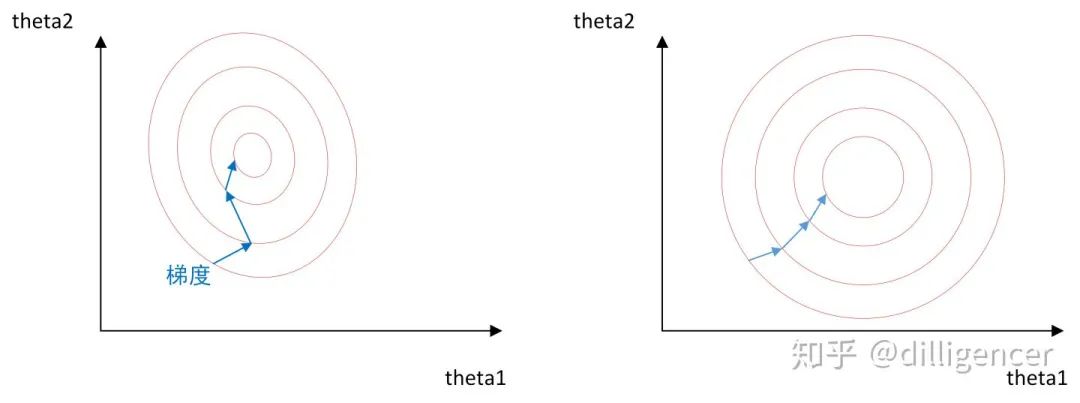
The image above represents the process of finding the optimal solution without normalization (left) and with normalization (right). When using gradient descent to seek the optimal solution, it is likely to take a zigzag path (moving vertically along the contour lines), leading to many iterations to converge; whereas the normalized contours appear more circular, allowing for faster convergence during gradient descent.
Thus, when machine learning models use gradient descent to seek optimal solutions, normalization is often very necessary; otherwise, convergence can be difficult or even impossible.
15. What types of normalization are there?
Applicable range: More suitable for cases where values are concentrated.
Disadvantages: If max and min are unstable, it easily leads to unstable normalization results, affecting subsequent usage.
2. Standard deviation normalization
Processed data conforms to a standard normal distribution, i.e., mean 0, standard deviation 1.
3. Nonlinear normalization
Applicable range: Often used in scenarios with large data variation, where some values are very large and others very small. This method includes log, exponentials, tangents, etc.
16. What is the effect of local response normalization?
LRN is a technique to improve the accuracy of deep learning. LRN is generally applied after activation and pooling functions.
-
a: Represents the output result after the convolution layer (including convolution and pooling operations), which is a four-dimensional array [batch,height,width,channel].
-
batch: batch size (each batch is one image).
-
-
-
channel: number of channels. This can be understood as the number of neurons output from a specific image after convolution or the depth of the processed image.
2. Represents a position in this output structure [a,b,c,d], which can be understood as a point at a certain height and width in a specific channel of a certain image, i.e., the point at height b and width c of the d-th channel of the a-th image.
-
N: The N in the formula in the paper represents the number of channels (channel).
-
a, n/2, k represent the input, depth_radius, bias in the function. The parameters k and n are hyperparameters, generally set
-
The summation direction is along the channel direction, i.e., the square sum of the values of each point is along the third dimension of channel in a, meaning the square sum of the points of n/2 channels before (minimum being the 0-th channel) and n/2 channels after (maximum being the d-1-th channel) (a total of n+1 points). The English annotation of the function also states that input is treated as d three-dimensional matrices, meaning that the number of channels in input is treated as the number of three-dimensional matrices, and the summation direction is also along the channel direction.
In AlexNet, the LRN layer was proposed to create a competitive mechanism for the local activity of neurons, making the larger responses relatively larger while suppressing the smaller feedback from other neurons, enhancing the model’s generalization ability.
17. Advantages of Batch Normalization (BN) algorithm
Batch normalization (BN) normalizes the data in the middle layers of the neural network.
-
Reduces the need for manual parameter selection. In some cases, dropout and L2 regularization parameters can be eliminated, or smaller L2 regularization constraint parameters can be adopted;
-
Reduces the requirements for learning rates. Now we can use initially large learning rates or choose smaller learning rates, and the algorithm can still quickly converge during training;
-
Local response normalization can be dispensed with. BN itself is a normalization network (local response normalization exists in AlexNet).
-
Disrupts the original data distribution, alleviating overfitting to some extent (literature suggests this can improve accuracy by 1%).
-
Reduces vanishing gradients, speeds up convergence, and improves training accuracy.
18. BN algorithm process
Below is the process of the BN algorithm during training
Input: Output result of the previous layer, learning parameters
1. Calculate the mean of the output data from the previous layer
m is the batch size of the training samples
2. Calculate the standard deviation of the output data from the previous layer
3. Normalize the data, obtaining
Where is a small value added to avoid division by zero.
4. Reconstruction, obtaining data after the above normalization process
Where are learnable parameters.
19. Comparison of Batch Normalization and Group Normalization
Batch Normalization: Allows various networks to be trained in parallel. However, normalizing dimensions can lead to some issues—the inaccuracies in batch statistics estimation cause errors in BN to increase rapidly as the batch size decreases. In training large networks and transferring features to computer vision tasks (including detection, segmentation, and video), memory consumption limits can only use small batches of BN.
Group Normalization: GN groups channels and computes the mean and variance within each group. GN’s calculations are independent of batch size, and its accuracy remains stable across various batch sizes.
20. Comparison of Weight Normalization and Batch Normalization
Both belong to parameter rewriting methods, but the approaches differ.
Weight Normalization normalizes the network weights W; Batch Normalization normalizes the input data of a certain layer in the network.
Weight Normalization has the following three advantages over Batch Normalization:
-
Weight Normalization accelerates the convergence of deep learning network parameters by rewriting the network weights W without introducing minbatch dependencies, making it suitable for RNN (LSTM) networks (Batch Normalization cannot be directly applied to RNNs because: 1) RNN processes sequences of variable lengths; 2) RNN computes based on time steps, and if Batch Normalization is used, it requires saving the mean and variance of each mini-batch at each time step, which is inefficient and memory-consuming).
-
Batch Normalization computes the mean and variance based on a mini-batch of data rather than the entire training set, introducing noise into gradient calculations. Therefore, Batch Normalization is unsuitable for noise-sensitive reinforcement learning and generative models (e.g., GANs, VAEs). In contrast, Weight Normalization rewrites weights W using scalar g and vector v, where the rewriting vector v is fixed, thus introducing less noise than Batch Normalization.
-
Weight Normalization does not require additional storage space to save the mean and variance of mini-batches. The additional computational overhead in performing forward signal propagation and backward gradient calculations during Weight Normalization is also minimal. Therefore, it is faster than performing normalization operations using Batch Normalization. However, Weight Normalization does not have the effect of keeping the output Y of each layer fixed within a range as Batch Normalization does. Thus, special attention must be paid to the choice of initial parameter values when using Weight Normalization.
21. When is Batch Normalization most suitable?
In CNNs, BN should be applied before nonlinear mappings. When training neural networks encounters slow convergence or gradient explosion, BN can be tried to resolve these issues. Additionally, BN can generally be added to speed up training and improve model accuracy.
BN is particularly suitable when each mini-batch is relatively large and the data distribution is close. Adequate shuffling should be performed before training; otherwise, the effect may be significantly worse. Moreover, since BN needs to statistically estimate first-order and second-order statistics of each mini-batch during operation, it is unsuitable for dynamic network structures and RNN networks.
22. What are the commonly used parameters for learning rate decay?
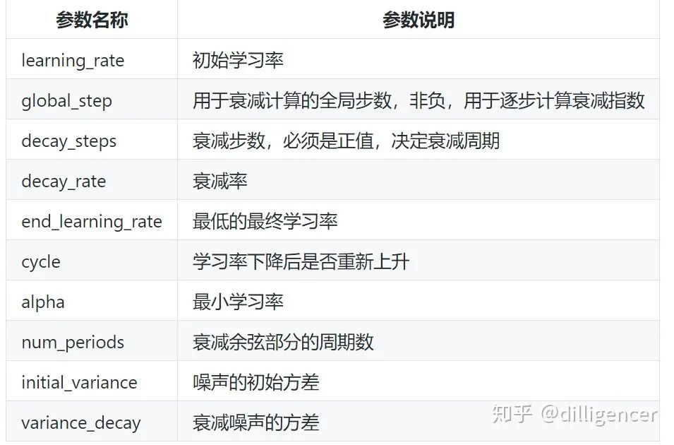
Deep learning may face overfitting issues—high variance, with two solutions: regularization and preparing more data. This is a very reliable method, but you may not always be able to prepare enough training data or the cost of obtaining more data is high. Regularization usually helps avoid overfitting or reduce your network error.
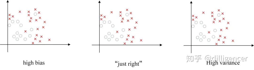
The left image shows high bias, the right image shows high variance, and the middle is Just Right.
24. Understanding dropout regularization
Do not rely on any single feature, as the input of that unit may be cleared at any time. Therefore, the unit propagates in this way and adds some weight to the four inputs of the unit. By propagating all weights, dropout will produce the effect of shrinking the square norm of the weights, similar to the previously discussed L2 regularization; implementing dropout effectively compresses weights and performs some outer regularization to prevent overfitting. L2 decay varies for different weights, depending on the size of the activation function’s multiplication.
25. Choosing dropout rates
1. Through cross-validation, the best dropout rate for hidden nodes is found to be 0.5, as this allows for the most random network structures to be generated.
2. Dropout can also be used as a method of adding noise, directly manipulating the input, with the input layer set to a value closer to 1, ensuring that input changes are not too large (0.8).
3. Performing spherical constraints (max-normalization) on the training of parameters w is very useful for dropout training.
4. Using pretraining methods can also assist in training parameters with dropout; when using dropout, all parameters should be multiplied by 1/p.
26. What are the drawbacks of dropout?
A major drawback of dropout is that the cost function J is no longer clearly defined; during each iteration, some nodes are randomly removed, making it difficult to retrospectively check the performance of gradient descent. A clearly defined cost function J decreases after each iteration because the cost function J we optimize is not clearly defined or is difficult to compute to a certain extent, so we lose debugging tools to plot such graphs. I usually turn off the dropout function, setting the keep-prob value to 1, run the code, and ensure that the J function monotonically decreases. Then I enable the dropout function, hoping that the code does not introduce bugs during dropout. I think you can also try other methods, although we do not have performance statistics on these methods, but you can use them in conjunction with dropout methods.
27. How to understand Internal Covariate Shift?
Why is training deep neural network models so difficult? One significant reason is that deep neural networks involve many layers of stacking, and the parameter updates of each layer cause changes in the input data distribution of the upper layers. Due to the stacking, the input distribution of the upper layers changes dramatically, making it necessary for the upper layers to constantly readjust to the parameter updates of the lower layers. To train the model well, we need to be very careful in setting the learning rate, initializing weights, and implementing detailed parameter update strategies.
Google summarized this phenomenon as Internal Covariate Shift, abbreviated as ICS. What is ICS?
It is well-known that a classic assumption in statistical machine learning is that the data distributions of the source domain and target domain are consistent. If they are not, it leads to new machine learning problems such as transfer learning/domain adaptation. Covariate shift is a branch of the inconsistent distribution hypothesis, referring to the condition where the conditional probabilities of the source and target domains are consistent, but their marginal probabilities differ.
Upon reflection, it is evident that for the outputs of the layers in a neural network, their distributions differ from the input signal distributions due to layer operations, and this difference increases with network depth. However, the sample labels (label) they can “indicate” remain unchanged, which aligns with the definition of covariate shift. Since it analyzes inter-layer signals, it is termed “internal”.
What problems does ICS cause?
In brief, the input data for each neuron is no longer “independently and identically distributed”.
First, upper layer parameters need to constantly adapt to new input data distributions, slowing down the learning process.
Second, the changes in lower layer inputs may tend to increase or decrease, leading upper layers to enter saturation zones, causing early termination of learning.
Third, the updates of each layer affect other layers, so the parameter update strategies for each layer need to be as cautious as possible.
Important! The Yi Zhen Natural Language Processing - Academic WeChat group has been established. You can scan the QR code below to join the group for discussions. Note: Please modify your remarks to [School/Company + Name + Direction] when adding. For example, --- Harbin Institute of Technology + Zhang San + Dialogue System. Please avoid adding if you are a WeChat merchant. Thank you!

Recommended Reading:
【Long Article Explanation】From Transformer to BERT Model
Sai'er Translation | Understanding Transformer from Scratch
A picture is worth a thousand words! A step-by-step guide to building a Transformer with Python