In-Depth Analysis of Convolutional Neural Networks (CNN)

This article summarizes some basic concepts of Convolutional Neural Networks (CNN) and provides a detailed explanation of the principles behind them. Through this article, you can gain a comprehensive understanding of Convolutional Neural Networks (CNN), which is very suitable as an introductory learning resource for deep learning.

Before we dive into the explanation, I have organized alearning roadmap for beginners in machine learning and deep learning, which includes specific content to belearned at each stage,tutorial videos for direct access,books and materials,time frames, andnoteworthy points.

If you lack direction in your studies, you can follow this roadmap, which can greatly save you time.

If you need this material, you can add my assistant to share it with you promptly and free of charge!

1. What is a Convolutional Neural Network

The concept of Convolutional Neural Networks (CNN) can be traced back to the 1980s and 1990s, but there was a period when this concept was “shelved” due to the limitations of hardware and software technology at that time. With the successive proposals of various deep learning theories and the rapid development of numerical computing devices, Convolutional Neural Networks have experienced rapid growth. So, what exactly is a Convolutional Neural Network? Taking handwritten digit recognition as an example, the entire recognition process is as follows:

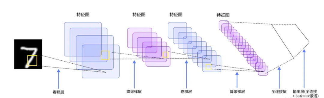
Figure 1: Handwritten Digit Recognition Process

The above process is the entire process of recognizing handwritten digits, and we can see that the entire process requires calculations at the following layers:

• Input Layer: Input image and other information

• Convolutional Layer: Used to extract the low-level features of the image

• Pooling Layer: Prevents overfitting and reduces data dimensionality

• Fully Connected Layer: Summarizes the low-level features and information obtained from the convolutional and pooling layers

• Output Layer: Obtains the most probable result based on the information from the fully connected layer

It can be seen that the most important layer among these is the convolutional layer, which is also the origin of the name Convolutional Neural Network. Below, I will explain the relevant content of these layers in detail.

2. Input Layer

The input layer is relatively simple. Its main job is to input image and other information, as Convolutional Neural Networks primarily deal with image-related content.

But are the images we see with our eyes the same as those processed by computers? Clearly, they are not. For the input image, we must first convert it into the corresponding two-dimensional matrix, which is composed of the pixel values of each pixel in the image.

We can look at an example, as shown in the following image of the handwritten digit “8”. After being read by the computer, the image is stored as a two-dimensional matrix composed of pixel values.

Figure 2: Grayscale Image of 8 and its Corresponding Two-Dimensional Matrix

The above image is also called a grayscale image because the range of each pixel value is from 0 to 255 (from pure black to pure white), indicating the intensity of its color.

There are also black and white images, where each pixel value is either 0 (indicating pure black) or 255 (indicating pure white).

The most common type we encounter in daily life is the RGB image, which has three channels: red, green, and blue. The range of each pixel value in each channel is also from 0 to 255, indicating the intensity of each pixel’s color.

However, we usually process mainly grayscale images because they are easier to handle (with a smaller range of values and simpler colors). Some RGB images are also converted to grayscale images before being input into the neural network for easier computation; otherwise, the computational load would be very high when processing all three channels together.

Of course, with the rapid development of computer performance, some neural networks can now also process three-channel RGB images.

Now we know that the role of the input layer is to convert the image into a two-dimensional matrix composed of pixel values and store this matrix for the operations of the subsequent layers.

3. Convolutional Layer

So how do we process the image once it is inputted?

Assuming we have obtained the two-dimensional matrix of the image and want to extract features from it, the convolution operation will assign a high value to regions where features exist and a low value otherwise.

This process is determined by calculating the product with the convolution kernel (Convolution Kernel).

Assuming our input image is a person’s head and the eyes are the features we want to extract, we will use the eyes as the convolution kernel and move it across the image of the person’s head to determine where the eyes are, as shown in the following process:

Figure 3: Process of Extracting Eye Features

Through the entire convolution process, we obtain a new two-dimensional matrix, which is also referred to as a feature map (Feature Map).

Finally, we can apply coloring to the obtained feature map (for example, high values could be white and low values could be black), allowing us to extract features related to the person’s eyes, as shown below:

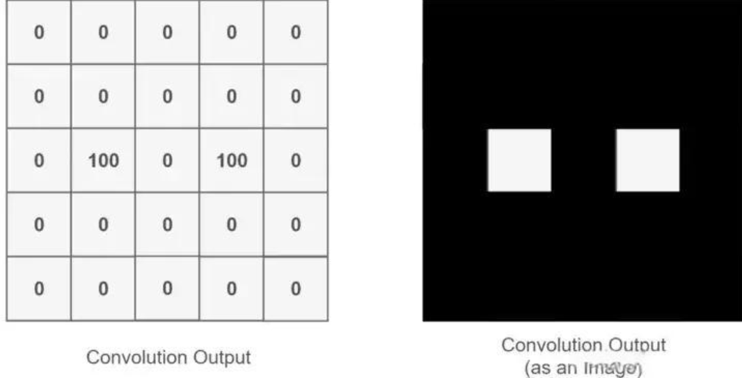
Figure 4: Result of Extracting Eye Features

The description above may seem a bit confusing; don’t worry. First, the convolution kernel is also a two-dimensional matrix, but it must be smaller than or equal to the size of the input image’s two-dimensional matrix. The convolution kernel moves continuously across the input image’s two-dimensional matrix, performing a multiplication and summation at each position, as shown in the diagram below:

Figure 5: Convolution Process

As we can see, the entire process is a dimensionality reduction process, where the continuous movement of the convolution kernel allows us to extract the most useful features from the image.

We usually refer to the new two-dimensional matrix obtained from the convolution kernel calculations as a feature map. For example, in the moving animation above, the dark blue square below is the convolution kernel, while the stationary cyan square above is the feature map.

Some readers may have noticed that every time the convolution kernel moves, the middle position is calculated multiple times, while the edges of the input image’s two-dimensional matrix are only calculated once. Wouldn’t this lead to inaccurate results?

Let’s think carefully. If the edges are calculated only once while the middle is calculated multiple times, the resulting feature map will lose edge features, ultimately leading to inaccurate feature extraction.

To solve this problem, we can expand the original two-dimensional matrix of the input image by one or more circles, allowing every position to be fairly calculated and not losing any features.

This process can be seen in the two situations below. This method of expanding to solve feature loss is known as Padding.

• Padding value of 1, expanding by one circle

Figure 6: Convolution Process with Padding of 1

• Padding value of 2, expanding by two circles

Figure 7: Convolution Process with Padding of 2

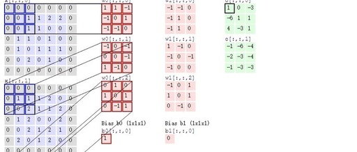
Now, what if the situation is more complex? If we use two convolution kernels to extract features from a color image? As mentioned earlier, color images consist of three channels, meaning a color image will have three two-dimensional matrices. For simplicity, we will only consider the first channel. At this point, we will use two sets of convolution kernels, each set used to extract features from its respective channel’s two-dimensional matrix. Since we are only considering the first channel, we only need to use the first convolution kernel from each set to compute the feature map, as shown in the following process:

Figure 8: Convolution Process with Two Convolution Kernels

Looking at the animation above, it might seem a bit overwhelming. Let me explain. Following the previous logic, the input image is a color image with three channels, so the input image size is 7×7×3.

Since we are only considering the first channel, we will extract features from the first 7×7 two-dimensional matrix using only the first convolution kernel from each set. You may notice the term Bias, which is simply the bias term; we just add it to the final computed result to obtain the feature map.

It can be observed that the number of feature maps corresponds to the number of convolution kernels used. Since we only used two convolution kernels, we will obtain two feature maps.

That covers some knowledge related to the convolutional layer. Of course, this article is just an introduction, so there are still some more complex topics that have not been discussed in depth, which will need to be covered in future learning and summaries.

4. Pooling Layer

As mentioned earlier, the number of feature maps corresponds to the number of convolution kernels, and in reality, the situation is certainly more complex, resulting in even more convolution kernels.

This means there will be more feature maps. When there are numerous feature maps, it implies that we have obtained a lot of features, but are all these features necessary?

Clearly not; many features may be unnecessary, and these extraneous features often lead to the following two problems:

• Overfitting

• High dimensionality

To solve this problem, we can utilize the pooling layer. So, what is the pooling layer?

The pooling layer, also known as down-sampling, means that after performing convolution operations, we extract the most representative features from the obtained feature maps, which can help reduce overfitting and lower dimensionality. This process is illustrated as follows:

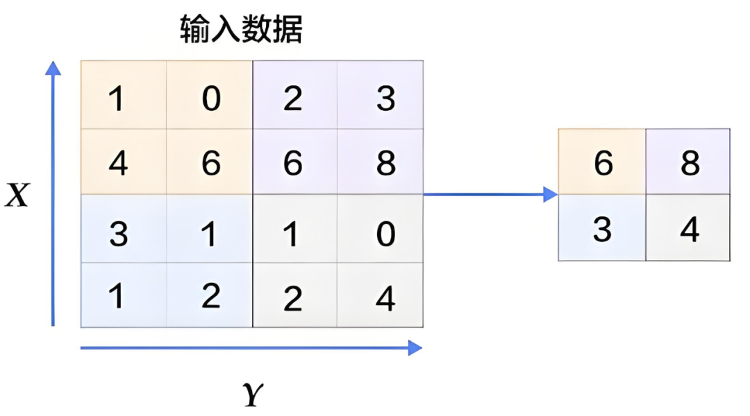
Figure 9: Pooling Process

You may ask how to determine the most representative features?

This process is similar to the convolution process, where a small square moves across the image, and we take the most representative feature from this square each time.

Now the question arises: how do we extract the most representative features? There are usually two methods:

• Max Pooling

As the name suggests, max pooling takes the maximum value from all values in the square, which represents the most representative feature at that position. This process is shown as follows:

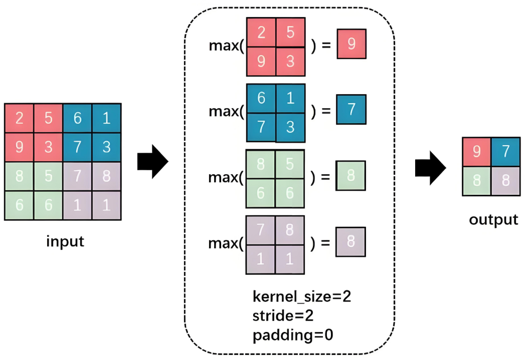
Figure 10: Max Pooling Process

There are a few parameters that need explanation:

① kernel_size = 2: The size of the square used in the pooling process is 2×2. If it were in the convolution process, it would mean the size of the convolution kernel is also 2×2.

② stride = 2: Each time the square moves two positions (from left to right, from top to bottom). This process is similar to the convolution operation.

③ padding = 0: This was explained earlier; if this value is 0, it means no expansion was performed.

• Average Pooling

Average pooling takes the average of all values in the square region, considering the influence of each position’s value on the feature. The average pooling calculation is also relatively simple, as shown in the following process:

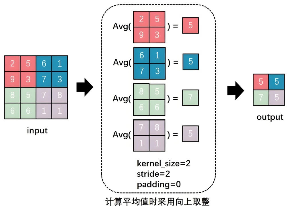
Figure 11: Average Pooling Process

The meanings of the parameters are consistent with those described for max pooling. Additionally, it is important to note that when calculating average pooling, rounding up is used.

The above is all the operations related to the pooling layer. Let’s review: after pooling, we can extract more representative features.

At the same time, we reduce unnecessary computations, which greatly benefits neural network calculations in real-world applications.

In reality, neural networks can be quite large, and after the pooling layer, the efficiency of the model can be significantly improved. Therefore, the pooling layer has many advantages, which can be summarized as follows:

• Reduces the number of parameters while preserving the original features of the image

• Effectively prevents overfitting

• Brings translation invariance to convolutional neural networks

The first two advantages have already been discussed. So, what is translation invariance? We can use one of our previous examples, as shown in the following image:

Figure 12: Pooling Translation Invariance As we can see, the positions of the two original images are different; one is normal while the other has the person’s head slightly shifted to the left.After convolution operations, we obtain their corresponding feature maps. The positions of the eye features in the two feature maps correspond to their original images; one is normal, while the other has the eye feature slightly shifted.While a human can distinguish this, neural network calculations might introduce errors, as the expected position of the eye feature may not appear. What should we do?At this point, using the pooling layer for pooling operations allows us to see that although the eye features of the two images were not in the same position before pooling, after pooling, the eye feature positions are the same. This facilitates subsequent calculations in the neural network. This property is called the translation invariance of pooling.5. Fully Connected LayerLet’s assume we are still using the example of the person’s head. Now that we have extracted the features of the eyes, nose, and mouth through convolution and pooling, how can we use these features to determine whether the image is of a person’s head?At this point, we simply need to “flatten” all the extracted feature maps, transforming their dimensions into 1 × x 1×x1×x. This process is known as the fully connected process.In other words, in this step, we expand all the features and perform calculations, ultimately obtaining a probability value that indicates the likelihood of the input image being that of a person’s head, as illustrated below:

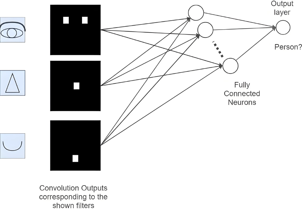
Figure 13: Fully Connected ProcessLooking at this process alone may still be unclear, so we can combine the previous processes with the fully connected layer, as shown in the diagram below:

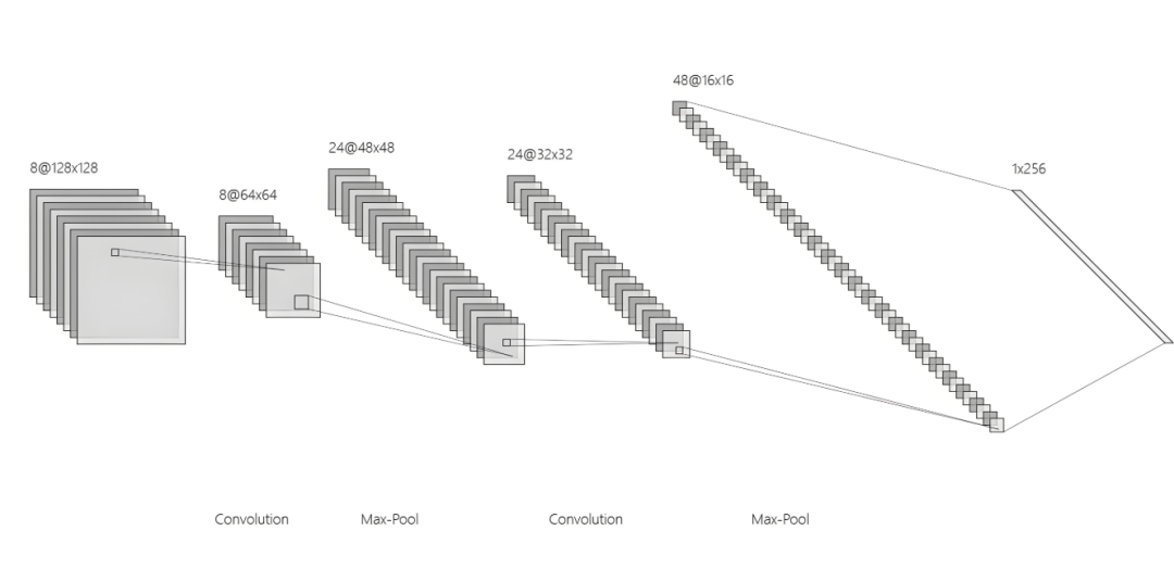
Figure 14: Overall Process

After two rounds of convolution and max pooling, we obtain the final feature map. At this point, the features are strong representatives of the input data. Finally, after passing through the fully connected layer and expanding to a one-dimensional vector, we perform one last calculation to obtain the final recognition probability. This is the entire process of a convolutional neural network.6. Output LayerThe output layer of a convolutional neural network is relatively straightforward. We simply need to calculate the recognition value’s probability from the one-dimensional vector obtained from the fully connected layer.Of course, this calculation may be linear or nonlinear.In deep learning, the results we typically need to recognize are usually multi-class outputs. Therefore, each position will have a probability value representing the likelihood of recognition as the current value. The position with the highest probability value is the final recognition result.During training, we can continuously adjust the parameter values to improve the accuracy of the recognition results, thereby achieving the highest model accuracy.

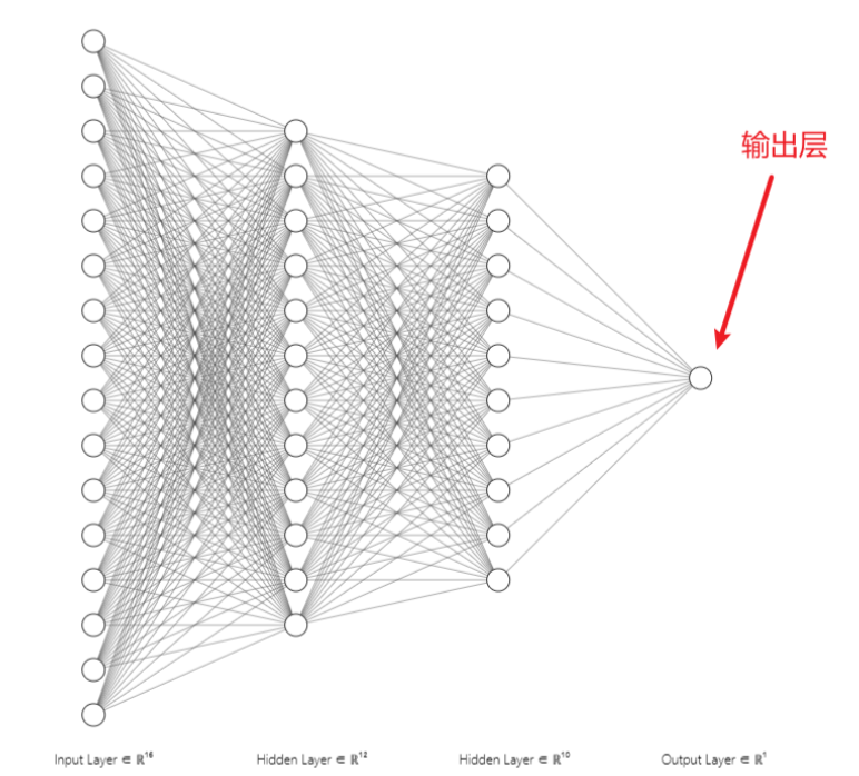
Figure 15: Output Layer Schematic7. Review of the Entire ProcessThe most classic application of convolutional neural networks is undoubtedly handwritten digit recognition. For instance, if I write the digit 8 by hand, how does the convolutional neural network recognize it? The entire recognition process is illustrated in the following diagram:

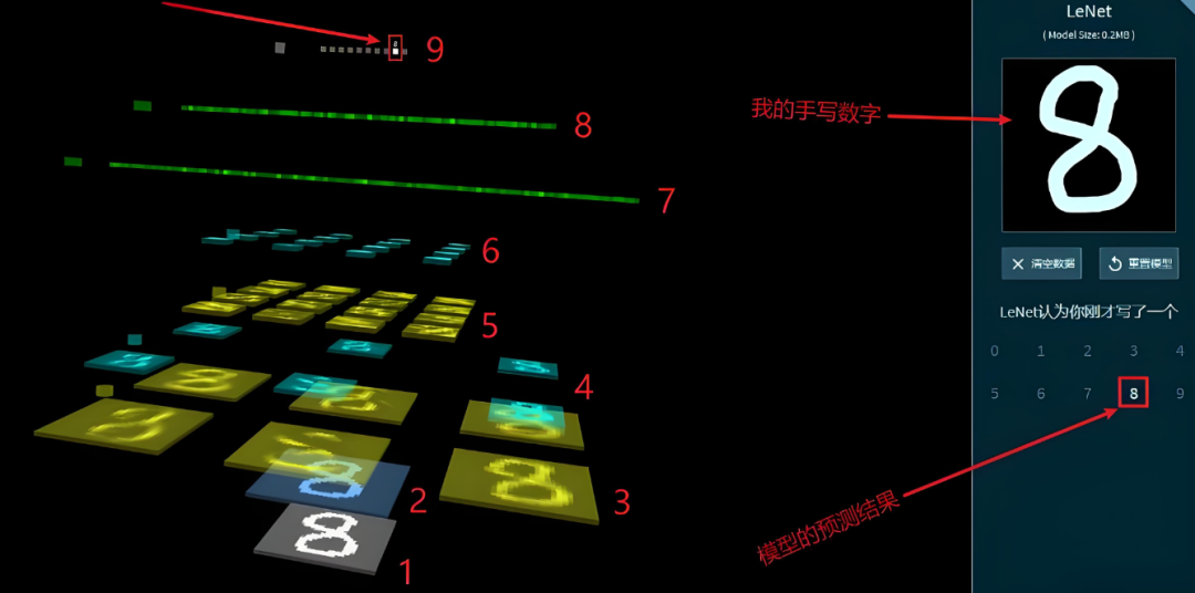
Figure 16: Handwritten Digit Recognition Process

1. Convert the handwritten digit image into a pixel matrix
2. Perform convolution operations on the pixel matrix with non-zero padding to preserve edge features and generate a feature map
3. Use six convolution kernels to perform convolution operations on this feature map, generating six feature maps
4. Perform pooling operations (also known as down-sampling) on each feature map while preserving features and reducing data flow, resulting in six smaller images that resemble the previous feature maps but with reduced dimensions
5. Perform a second round of convolution operations on the six smaller images obtained from pooling, generating more feature maps
6. Perform pooling operations (down-sampling) on the feature maps generated in the second round of convolution
7. Conduct the first fully connected operation on the features obtained from the second pooling operation
8. Conduct the second fully connected operation on the results from the first fully connected operation
9. Finally, perform one last operation on the results from the second fully connected operation, which may be linear or nonlinear. Each position (a total of ten positions, from 0 to 9) will have a probability value representing the likelihood of recognizing the input handwritten digit as the current digit. The position with the highest probability value is taken as the recognition result. As can be seen on the upper left side of the image, the model (LeNet) successfully recognized the handwritten digit, as indicated by the final result on the left side of the image.