CNN: Convolutional Neural Network – Convolutional Neural Network
RNN: Recurrent Neural Network – Recurrent Neural Network
DNN: Deep Neural Networks – Deep Neural Networks
First, let’s talk about DNN. Structurally, it is similar to traditional NN (Neural Networks), but the development of neural networks encountered some bottleneck issues.
Initially, neurons could not represent the XOR operation. Scientists found that by increasing the number of layers and hidden layers, they could express it. They discovered that the number of layers in a neural network directly determines its ability to express reality. However, as the number of layers increases, local functions are more likely to reach a local optimum, and training a deep network with data sometimes performs worse than a shallow network, leading to the problem of gradient vanishing.
We often use the sigmoid function as the input-output function of neurons. When the signal of 1 is passed to the next layer during backpropagation, it becomes 0.25, making it almost impossible to adjust parameters in the last few layers. It is worth mentioning that the recently proposed highway networks and deep residual learning avoid the problem of gradient vanishing.
The main difference between DNN and NN is that the sigmoid function is replaced with ReLU and maxout, overcoming the gradient vanishing issue.
The image below shows the structure of a deep network DNN.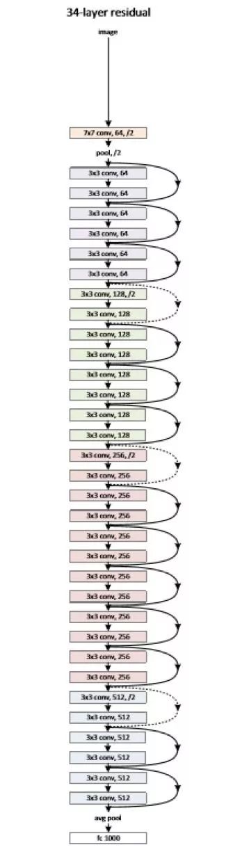
The depth of deep learning does not have a fixed definition. In 2006, Hinton solved the problem of local optimum by developing the hidden layer to 7 layers, which reached what is referred to as true depth in deep learning. The number of hidden layers required to solve different problems varies; generally, 4 layers suffice for speech recognition, while 20 layers are common for image recognition. However, as the number of layers increases, the problem of parameter explosion arises. Assuming the input image is 1K*1K, there would be 1M nodes in the hidden layer, resulting in 10^12 weights to adjust, which can easily lead to overfitting and local optimum issues. To address these problems, CNN was proposed.
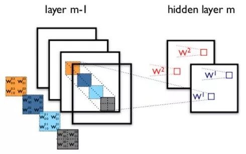
CNN maximally utilizes the local information in images. There are inherent local patterns in images (such as contours, edges, and features like eyes, noses, and mouths) that can be leveraged. It is clear that the concepts in image processing should be combined with neural network technology. In CNN, not all neurons in adjacent layers are directly connected; instead, they connect through a “convolution kernel” as an intermediary. The same convolution kernel is shared across all images, and after convolution, the original positional relationships are preserved. The hidden layers of the convolutional neural network can be simply illustrated through an example. Assume m-1=1 is the input layer, and we need to recognize a color image that has four channels ARGB (transparency and RGB, corresponding to four images of the same size). Let’s assume the convolution kernel size is 100*100, and we use 100 convolution kernels from w1 to w100 (intuitively, each convolution kernel should learn different structural features). Using w1 on the ARGB image for convolution can yield the first image of the hidden layer; the top-left pixel of this hidden image is the weighted sum of the pixels in the top-left 100*100 area of the four input images, and so on. Similarly, considering other convolution kernels, the hidden layer corresponds to 100 “images”. Each image represents a response to different features in the original image. Continuing this structure allows for further processing. CNN also includes operations like max-pooling to enhance robustness.
A typical structure of a convolutional neural network is observed, noting that the last layer is actually a fully connected layer. In this example, we see that the number of parameters from the input layer to the hidden layer decreases significantly, allowing us to obtain a good model using existing training data. This is suitable for image recognition; precisely because the model restricts the number of parameters and exploits local structures, following the same logic, CNN can also be applied to speech recognition by utilizing local information in speech spectrogram structures.
The structure of CNN is shown below:
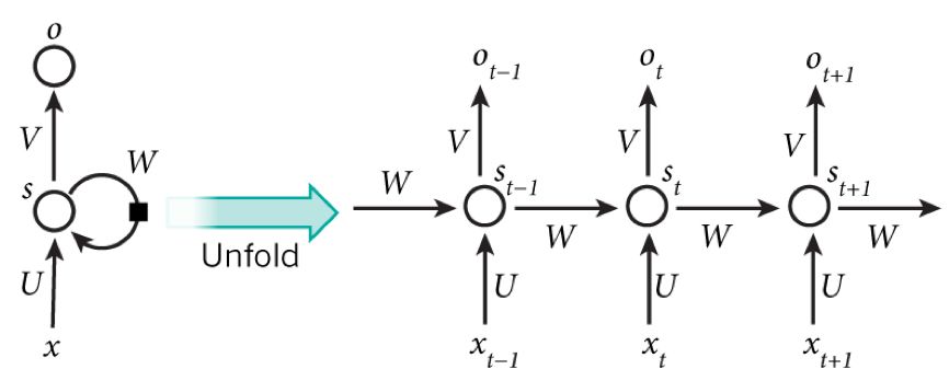
The fully connected DNN also has another problem—it cannot model changes over time series. However, the temporal order of sample occurrences is crucial for applications like natural language processing, speech recognition, and handwriting recognition. To meet this demand, another neural network structure emerged—Recurrent Neural Network RNN. In a typical fully connected network or CNN, the signals of neurons in each layer can only propagate to the layer above, and the processing of samples at various times is independent, thus they are also known as feed-forward neural networks. In RNN, the output of a neuron can directly affect itself at the next timestamp; that is, the input of the i-th layer neuron at time m includes not only the output of the (i-1) layer neuron at that time but also its own output at (m-1) time! This can be represented graphically as follows:

We can see that interconnections have been added between the hidden layer nodes. For ease of analysis, we often unfold RNN over time, resulting in the structure shown in the figure.
RNN can be viewed as a neural network that transmits over time; its depth is the length of time! Just as we mentioned earlier, the “gradient vanishing” phenomenon is likely to occur again, but this time it happens along the time axis. For time t, the gradient it produces vanishes after propagating a few layers along the time axis, making it unable to influence the distant past. Therefore, the previously mentioned “all history” working together is only an ideal situation; in practice, this influence can only last for several timestamps. To address the gradient vanishing over time, the field of machine learning has developed Long Short-Term Memory units.
Source: Feng Xiao Yi Shui Han – Blog Garden
http://www.cnblogs.com/softzrp/p/6434282.html
About Imagination WeChat Account
Authoritative news about Imagination’s CPU, GPU, and connectivity IP, wireless IP latest updates, providing information on applications such as IoT, wearables, communications, automotive electronics, and medical electronics. Daily updates of a large amount of information keep you updated on technological developments. Feel free to follow us! Just give a little tap on the QR code, and we’ll be good friends!