Implementing Image Inpainting with TensorFlow and Deep Learning

Big Data Digest article, see the end of the article for reposting requirements

Author | Brandon Amos

Translation | Molly, Han Xiaoyang

■ Introduction

■ Step 1: Understanding Images as Samples from a Probability Distribution

How do you fill in missing information?

But how do you start with statistics? These are all images.

So how do we fill in images?

■ Step 2: Quickly Generating Fake Images

Learning to generate new samples under an unknown probability distribution

[ML-Heavy] Architecture of Generative Adversarial Networks (GAN)

Using G(z) to generate pseudo-images

[ML-Heavy] Training DCGAN

Existing implementations of GAN and DCGAN

[ML-Heavy] Building DCGANs on TensorFlow

Running DCGAN on image datasets

■ Step 3: Finding the Best Pseudo-Images for Image Inpainting

Using DCGAN for image inpainting

[ML-Heavy] Loss function for projection to pgpg

[ML-Heavy] Using TensorFlow for DCGAN image inpainting

Filling in the images

■ Conclusion

Content-aware fill (note: Content-aware fill is a feature of Photoshop) is a powerful tool that designers and photographers can use to fill in unwanted or missing parts of images. When filling in missing or damaged parts of an image, image inpainting and repair are two closely related techniques. There are many methods to achieve content-aware fill, image inpainting, and repair. In this blog, I will introduce a paper by Raymond Yeh and Chen Chen, “Semantic Image Inpainting with Perceptual and Contextual Losses”. The paper was published on arXiv on July 26, 2016, and describes how to use the DCGAN network for image inpainting. This blog is aimed at readers with a general technical background, and some sections require a background in machine learning. I have marked the relevant sections with the [ML-Heavy] tag; if you do not want to delve into too much detail, you can skip these sections. We will only cover the case of filling in missing parts of facial images. The relevant TensorFlow code has been published on GitHub: bamos/dcgan-completion.tensorflow. Image inpainting is divided into three steps.

• First, we understand the image as a sample from a probability distribution.

• Based on this understanding, we learn how to generate pseudo-images.

• Then we find the pseudo-image that is best suited for filling in.

Using Photoshop to fill in missing parts of the image and using Photoshop to automatically remove unwanted parts.

The following will introduce image inpainting. The center of the image is generated automatically. The source code can be downloaded from here. These images are a random sample taken from the LFW dataset.

1. How do you fill in missing information?

In the example above, imagine you are constructing a system that can fill in the missing parts. How would you do it? How do you think the human brain does it? What kind of information do you use? In this blog, we will focus on two types of information: contextual information: you can infer information about the missing pixels from the surrounding pixels. Perceptual information: you fill in with “normal” parts, like how you see it in real life or other images. Both are important. Without contextual information, how do you know which one to fill in? Without perceptual information, countless possibilities can be generated through the same context. Some machine learning systems may produce images that look “normal” to machines, but may not seem quite right to humans. If there were a precise and intuitive algorithm that could capture the two properties mentioned in the previous image inpainting steps, it would be perfect. Constructing such an algorithm is feasible for specific cases. However, there is currently no general method. The best solution is to obtain an approximate technique through statistics and machine learning.

2. But how do you start with statistics? These are all images.

To stimulate everyone’s thinking, we start with a well-understood probability distribution that can be expressed in a concise form: a normal distribution. This is the probability density function (PDF) of the normal distribution. You can think of the PDF as moving horizontally across the input space, with the vertical axis representing the probability of a certain value occurring. (If you’re interested, the code to draw this graph can be downloaded from bamos/dcgan-completion.tensorflow:simple-distributions.py.)

Sampling from this distribution gives you some data. It is important to clarify the relationship between the PDF and the samples.

Sampling from a normal distribution

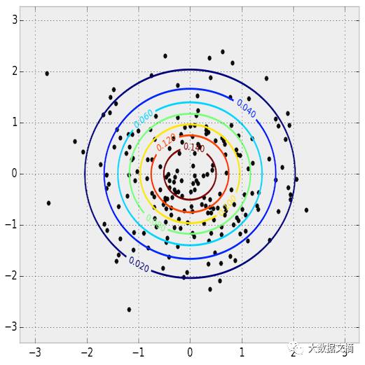
2D image PDF and sampling. PDF is represented with contour plots, and sample points are drawn on top.

This is a 1D distribution because the input can only move along one dimension. The same can be done in two dimensions. The key connection between images and statistics is that we can think of images as samples obtained from a high-dimensional probability distribution. The probability distribution corresponds to the pixels of the image. Imagine you are taking a photo with a camera. The resulting image consists of a finite number of pixels. When you take a photo with the camera, you are sampling from this complex probability distribution. This probability distribution determines whether we judge an image to be normal or abnormal. Unlike the normal distribution, we cannot know the true probability distribution for images; we can only collect samples. In this article, we will use color images, which are represented using RGB colors. Our image is 64 pixels wide and 64 pixels high, so our probability distribution is 64⋅64⋅3≈12k dimensional.

3. So how do we fill in the image?

First, consider the multivariate normal distribution to seek some inspiration. Given x=1, what is the most likely value of y? We can fix the value of x and then find the y that maximizes the PDF.

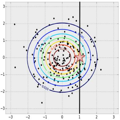
In a multivariate normal distribution, given x, obtain the maximum possible y

This concept can be naturally extended to image probability distributions. We know some values and want to fill in the missing values. This can be simply understood as a maximization problem. We search for all possible missing values, and the image used for filling is the one with the highest probability. From the samples of the normal distribution, we can derive the PDF just through the samples. Just pick your favorite statistical model and fit the data. However, we are not actually using this method. For simple distributions, the PDF is easy to derive. But for more complex image distributions, it becomes very difficult and challenging to handle. The complexity arises partly from complex conditional dependencies: the value of a pixel depends on the values of other pixels in the image. Moreover, maximizing a general PDF is a very difficult and tricky non-convex optimization problem.

1. Learning to generate new samples under an unknown probability distribution

Aside from learning how to compute the PDF, another mature idea in statistics is to learn how to use a generative model to generate new (random) samples. Generative models are generally difficult to train and handle, but later, the deep learning community made an amazing breakthrough in this area. Yann LeCun has provided a brilliant discussion on how to train generative models in this Quora answer, referring to it as one of the most interesting ideas in the field of machine learning in the past decade.

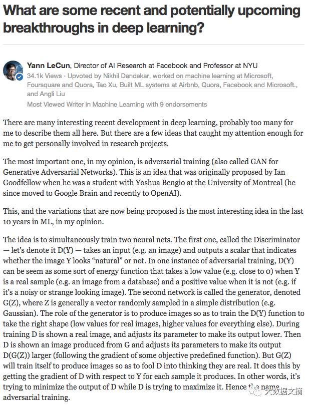
Yann LeCun’s introduction to Generative Adversarial Networks

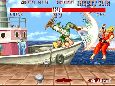
Generative Adversarial Networks can be likened to arcade games. Two networks compete against each other, progressing together, just like two humans competing in a game.

Other deep learning methods, such as Variational Autoencoders (VAEs), can also be used to train generative models. In this blog, we use Generative Adversarial Networks (GANs).

2. [ML-Heavy] Architecture of Generative Adversarial Networks (GAN)

This idea was proposed in the groundbreaking paper “Generative Adversarial Networks” (GANs) by Ian Goodfellow et al., presented at the 2014 Neural Information Processing Systems (NIPS) workshop. The main idea is to define a simple, commonly used distribution, represented as pz. In the following, we use pz to denote the uniform distribution on the closed interval [-1, 1]. We will denote a sample from this distribution as z∼pz. If pz is five-dimensional, we can sample it with a single line of Python code using numpy:

z = np.random.uniform(-1, 1, 5)

array([0.77356483, 0.95258473, -0.18345086, 0.69224724, -0.34718733])

Now that we have a simple distribution for sampling, we define a function G(z) to sample from our original probability distribution.

def G(z):

…

return imageSample

z = np.random.uniform(-1, 1, 5)

imageSample = G(z)

So how do we define G(z) to take a vector as input and output an image? We will use a deep neural network. There are many tutorials on the fundamentals of neural networks, so I won’t cover them here. Some good references include the Stanford CS231n course, Ian Goodfellow et al.’s Deep Learning book, Image Kernels Explained Visually, and the Convolution Arithmetic Guide.

There are many ways to construct a G(z) based on deep learning. The original GAN paper proposed an idea, a training process, and some preliminary experimental results. This idea has been greatly developed, one of which is presented in the paper “Unsupervised Representation Learning with Deep Convolutional Generative Adversarial Networks” by Alec Radford, Luke Metz, and Soumith Chintala, published at the 2016 International Conference on Learning Representations (ICLR). This paper proposed Deep Convolutional GANs (called DCGANs), using fractional stride convolutions to upsample images.

So what are fractional stride convolutions, and how do they upsample images? Vincent Dumoulin and Francesco Visin’s paper “A Guide to Convolution Arithmetic for Deep Learning” and the convolution arithmetic project provide a very good introduction to convolutions in deep learning. The illustrations are excellent and give us an intuitive understanding of how fractional stride convolutions work. First, make sure you understand how a standard convolution slides the kernel over the input space (in blue) to obtain the output space (in green). Here, the output is smaller than the input. (If you don’t understand, refer to the CS231n CNN section or the Convolution Arithmetic Guide)

Illustration of convolution operations, where blue is the input and green is the output.

Next, suppose you have a 3×3 input. Our goal is to upsample (upsample), resulting in a larger output. You can think of fractional stride convolutions as enlarging the input image and then inserting 0s between the pixels. Then, perform convolution operations on this enlarged image to obtain a larger output. Here, the output is 5×5.

Illustration of fractional stride convolution operations, where blue is the input and green is the output.

Note: The layers that perform upsampling have many names: full convolution, in-network upsampling, fractional stride convolution, backward convolution, deconvolution, up-convolution, or transposed convolution. It is highly discouraged to use the term “deconvolution” because it has other meanings: in certain mathematical operations and in other applications in computer vision, this term has entirely different meanings.

Now that we have the fractional stride convolution structure, we can express G(z) as taking a vector z∼pz as input and outputting a 64x64x3 RGB image.

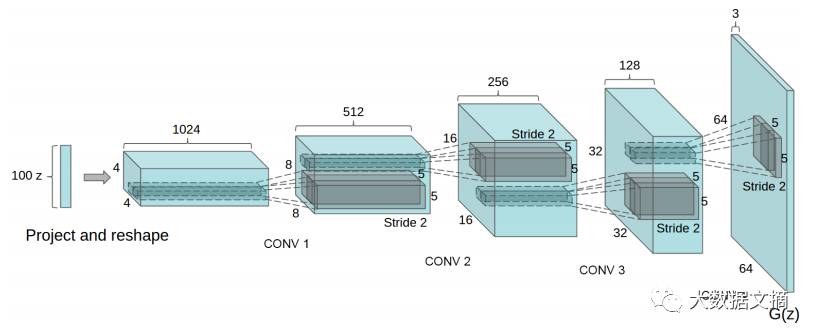
One way to construct a generator using DCGAN. The image is from the DCGAN paper.

The DCGAN paper also proposed other techniques and adjustments for training DCGANs, such as batch normalization and leaky ReLUs.

3. Using G(z) to Generate Pseudo-Images

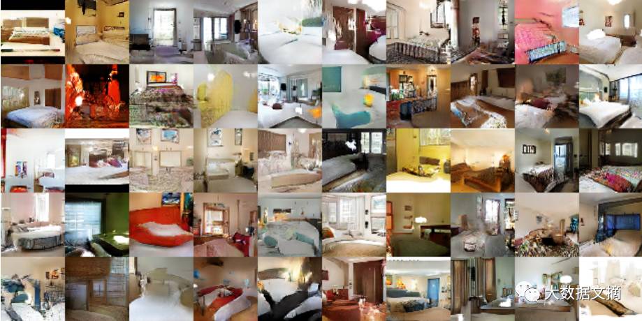
Let’s take a moment to appreciate how powerful G(z) is! The DCGAN paper shows how DCGAN can train on the bedroom dataset. Then G(z) can produce the following pseudo-images, representing what the generator thinks a bedroom looks like. None of the images below are in the original dataset!

Additionally, you can perform algebraic operations in the input space z. Below is a network that generates faces.

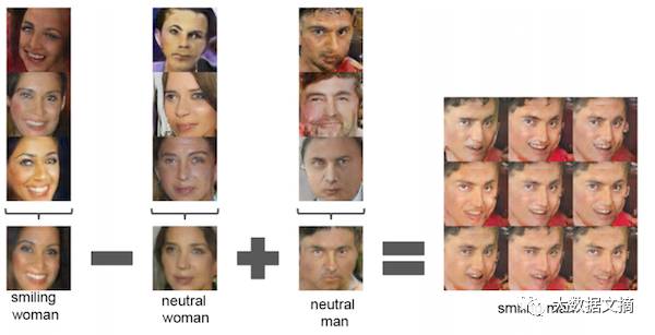
Face algebra operations based on DCGAN. Image from the DCGAN paper.

4. [ML-Heavy] Training DCGAN

Now that we have defined G(z) and seen how powerful it is, how do we train it? We have many unknown variables (parameters) that we need to find. At this point, we need to use adversarial networks. First, we need to define some symbols. The probability distribution of the data (unknown) is denoted as pdata. Then G(z), (where z∼pz) can be understood as sampling from a probability distribution. Let’s denote this probability distribution as pg.

The symbols pz, pdata, pg mean the probability distribution of z, a simple, known image probability distribution (unknown), which is the source of image data samples for the generator G to sample from, and we hope pg==pdata. The symbol pz indicates the probability distribution of z, a simple, known pdata image probability distribution (unknown), which is the source of image data samples for the generator G to sample from, and we hope pg==pdata.

The discriminator network D(x) takes an image x as input and returns the probability that the image x is sampled from the distribution pdata. Theoretically, when the input image is sampled from pdata, the discriminator outputs a value close to 1, while when the input image is a pseudo-image, such as one sampled from pg, the discriminator outputs a value close to 0. In DCGANs, D(x) is a traditional convolutional neural network.

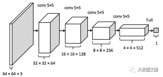
The discriminator convolutional neural network, image from the image recovery paper

The goal of training the discriminator is:

· 1. For each image from the real data distribution x∼pdata, maximize D(x).

· 2. For each image that is not from the real data distribution x≁pdata, minimize D(x).

The generator G(z)’s training goal is to generate samples that can confuse D. The output is an image that can be used as input to the discriminator. Therefore, the generator wants to maximize D(G(z)), which is equivalent to minimizing (1-D(G(z))), since D is a probability that takes values between 0 and 1.

The paper proposes that the adversarial network is realized through the following min-max strategy. The expectation in the first term traverses the real data distribution, while the expectation in the second term traverses samples from pz, which is equivalent to traversing G(z)∼pg.

minGmaxDEx∼pdatalog(D(x)+Ez∼pz[log(1−D(G(z)))

Through this expression, we can train the parameters of D and G. We know how to quickly compute each part of this expression. The expectation can be estimated with a small batch of size m, and the inner maximization can be estimated with k steps of gradients. It has been proven that k=1 is a suitable value for training.

We denote the parameters of the discriminator as θd and the parameters of the generator as θg. The gradients of the losses with respect to θd and θg can be computed through backpropagation since D and G are both composed of mature neural network modules. Below is the training strategy from the GAN paper. Theoretically, after training, pg==pdata. Therefore, G(z) can generate samples that follow the pdata distribution.

The training algorithm from the GAN paper.

5. Existing Implementations of GAN and DCGAN

On GitHub, you can find many great GAN and DCGAN implementations. goodfeli/adversarial: Theano GAN implementation by the authors of the GAN paper. tqchen/mxnet-gan: Unofficial MXNet GAN implementation. Newmu/dcgan_code: Theano GAN implementation by the authors of the DCGAN paper. soumith/dcgan.torch: Torch DCGAN implementation by one of the authors of the DCGAN paper (Soumith Chintala). carpedm20/DCGAN-tensorflow: Unofficial TensorFlow DCGAN implementation. openai/improved-gan: Code behind OpenAI’s first paper. There have been many modifications based on carpedm20/DCGAN-tensorflow. mattya/chainer-DCGAN: Unofficial Chainer DCGAN implementation. jacobgil/keras-dcgan: Unofficial (unfinished) Keras DCGAN implementation.

We will build our model based on carpedm20/DCGAN-tensorflow.

6. [ML-Heavy] Building DCGANs on TensorFlow

This implementation is in my bamos/dcgan-completion.tensorflow GitHub repository. I need to emphasize that this part of the code comes from Taehoon Kim’s carpedm20/DCGAN-tensorflow. I use it in my own repository for convenience in using it in the next part of image inpainting.

Most of the implementation code is in a Python class in model.py in DCGAN. Putting everything into a class has many benefits, allowing us to retain the intermediate process after training and load it for later use.

First, we define the generator and discriminator structures. The linear, conv2d_transpose, conv2d, and lrelu functions are defined in ops.py .

def generator(self, z):

self.z_, self.h0_w, self.h0_b = linear(z, self.gf_dim*8*4*4, ‘g_h0_lin’, with_w=True)

self.h0 = tf.reshape(self.z_, [-1, 4, 4, self.gf_dim * 8])

h0 = tf.nn.relu(self.g_bn0(self.h0))

self.h1, self.h1_w, self.h1_b = conv2d_transpose(h0,

[self.batch_size, 8, 8, self.gf_dim*4], name=’g_h1′, with_w=True)

h1 = tf.nn.relu(self.g_bn1(self.h1))

h2, self.h2_w, self.h2_b = conv2d_transpose(h1,

[self.batch_size, 16, 16, self.gf_dim*2], name=’g_h2′, with_w=True)

h2 = tf.nn.relu(self.g_bn2(h2))

h3, self.h3_w, self.h3_b = conv2d_transpose(h2,

[self.batch_size, 32, 32, self.gf_dim*1], name=’g_h3′, with_w=True)

h3 = tf.nn.relu(self.g_bn3(h3))

h4, self.h4_w, self.h4_b = conv2d_transpose(h3,

[self.batch_size, 64, 64, 3], name=’g_h4′, with_w=True)

return tf.nn.tanh(h4)

def discriminator(self, image, reuse=False):

if reuse:

tf.get_variable_scope().reuse_variables()

h0 = lrelu(conv2d(image, self.df_dim, name=’d_h0_conv’))

h1 = lrelu(self.d_bn1(conv2d(h0, self.df_dim*2, name=’d_h1_conv’)))

h2 = lrelu(self.d_bn2(conv2d(h1, self.df_dim*4, name=’d_h2_conv’)))

h3 = lrelu(self.d_bn3(conv2d(h2, self.df_dim*8, name=’d_h3_conv’)))

h4 = linear(tf.reshape(h3, [-1, 8192]), 1, ‘d_h3_lin’)

return tf.nn.sigmoid(h4), h4

When we initialize this class, we will use these two functions to build the model. We need two discriminators that share (reuse) parameters. One is for the small batch of images from the data distribution, and the other is for the small batch of images generated by the generator.

self.G = self.generator(self.z)

self.D, self.D_logits = self.discriminator(self.images)

self.D_, self.D_logits_ = self.discriminator(self.G, reuse=True)

Next, we define the loss functions. Here we do not use summation, but rather the cross-entropy between D’s predicted values and the real values, as it is more useful. The discriminator hopes the predictions for all “real” data are 1, and for all the “fake” data generated by the generator are 0. The generator hopes the discriminator predicts both as 1.

self.d_loss_real = tf.reduce_mean(

tf.nn.sigmoid_cross_entropy_with_logits(self.D_logits,

tf.ones_like(self.D)))

self.d_loss_fake = tf.reduce_mean(

tf.nn.sigmoid_cross_entropy_with_logits(self.D_logits_,

tf.zeros_like(self.D_)))

self.g_loss = tf.reduce_mean(

tf.nn.sigmoid_cross_entropy_with_logits(self.D_logits_,

tf.ones_like(self.D_)))

self.d_loss = self.d_loss_real + self.d_loss_fake

We gather the variables of each model so that they can be trained separately.

t_vars = tf.trainable_variables()

self.d_vars = [var for var in t_vars if ‘d_’ in var.name]

self.g_vars = [var for var in t_vars if ‘g_’ in var.name]

Now we start optimizing the parameters using the ADAM optimizer. It is an adaptive non-convex optimization method that is very competitive against SGD and generally does not require manual tuning of the learning rate, momentum, and other hyperparameters.

d_optim = tf.train.AdamOptimizer(config.learning_rate, beta1=config.beta1) \
.minimize(self.d_loss, var_list=self.d_vars)

g_optim = tf.train.AdamOptimizer(config.learning_rate, beta1=config.beta1) \
.minimize(self.g_loss, var_list=self.g_vars)

Next, we iterate over the data. In each iteration, we sample a small batch of data and then use the optimizer to update the network. Interestingly, if G is updated only once, the discriminator’s loss does not go to zero. Additionally, I think the final calls to d_loss_fake and d_loss_real perform some unnecessary calculations since those values have already been computed in d_optim and g_optim. As a connection to TensorFlow, you could try optimizing this part and send a PR to the original repo.

for epoch in xrange(config.epoch):

…

for idx in xrange(0, batch_idxs):

batch_images = …

batch_z = np.random.uniform(-1, 1, [config.batch_size, self.z_dim]) \
.astype(np.float32)

# Update D network

_, summary_str = self.sess.run([d_optim, self.d_sum],

feed_dict={ self.images: batch_images, self.z: batch_z })

# Update G network

_, summary_str = self.sess.run([g_optim, self.g_sum],

feed_dict={ self.z: batch_z })

# Run g_optim twice to make sure that d_loss does not go to zero (different from paper)

_, summary_str = self.sess.run([g_optim, self.g_sum],

feed_dict={ self.z: batch_z })

errD_fake = self.d_loss_fake.eval({self.z: batch_z})

errD_real = self.d_loss_real.eval({self.images: batch_images})

errG = self.g_loss.eval({self.z: batch_z})

Done! Of course, the complete code will have more comments, which can be found in model.py.

7. Running DCGAN on Image Datasets

If you skipped the previous section but want to run the code, this part of the code is in the bamos/dcgan-completion.tensorflow GitHub repository. I want to emphasize again that this code comes from Taehoon Kim’s carpedm20/DCGAN-tensorflow. We use my repository here for convenience in the next step. Warning: If you do not have a GPU that supports CUDA, training this network will be very slow.

First, clone my bamos/dcgan-completion.tensorflow GitHub repository and OpenFace locally. We will use the Python-only part of OpenFace for image preprocessing. Don’t worry, you don’t need to install OpenFace’s Torch dependencies. Create a new directory and clone the following resource repositories.

git clone https://github.com/cmusatyalab/openface.git

git clone https://github.com/bamos/dcgan-completion.tensorflow.git

Next, install OpenCV and the dlib that supports python2. If you’re interested, you can try to implement dlib support for python3. There are some tricks during installation, and I wrote some notes in the OpenFace setup guide, including which version I installed and how to install it. Next, install the OpenFace Python library so we can preprocess the images. If you are not using a virtual environment, you need to use sudo for global installation when running setup.py. (If this part is difficult for you, you can also use OpenFace’s Docker installation.)

Next, download a facial image dataset. It doesn’t matter if the dataset is unlabeled; we will delete it. The incomplete list includes: MS-Celeb-1M, CelebA, CASIA-WebFace, FaceScrub, LFW, and MegaFace. Place the images in the directory dcgan-completion.tensorflow/data/your-dataset/raw to indicate that it is the raw data of the dataset.

Now we use OpenFace’s alignment tool to preprocess the images into 64X64 data.

./openface/util/align-dlib.py data/dcgan-completion.tensorflow/data/your-dataset/raw align innerEyesAndBottomLip data/dcgan-completion.tensorflow/data/your-dataset/aligned –size 64

Finally, we will flatten the directory of processed images so that there are only images and no subfolders in the directory.

cd dcgan-completion.tensorflow/data/your-dataset/aligned

find . -name ‘*.png’ -exec mv {} . \
find . -type d -empty -delete

cd ../../..

Now we can train the DCGAN. Install TensorFlow, and start training.

./train-dcgan.py –dataset ./data/your-dataset/aligned –epoch 20

You can check what the samples from the generator look like in the sample folder. I trained on the CASIA-WebFace dataset and the FaceScrub dataset because I had both datasets on hand. After 14 rounds of training, my samples looked like this.

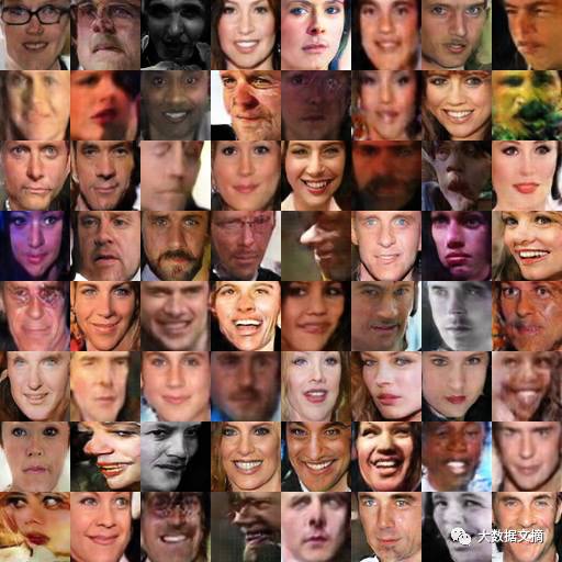
Samples from the DCGAN after 14 rounds of training on CASIA-WebFace and FaceScrub

You can also view TensorFlow images and loss functions on TensorBoard.

tensorboard –logdir ./logs

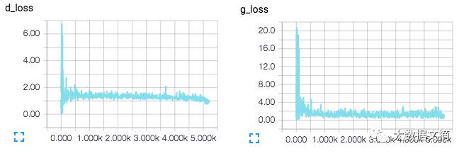
TensorBoard loss visualization image. Updated in real-time during training.

TensorBoard visualization of the DCGAN network

1. Using DCGAN for Image Inpainting

Now that we have the discriminator D(x) and generator G(z), how do we use them for image inpainting? In this chapter, I will introduce a paper by Raymond Yeh and Chen Chen, “Semantic Image Inpainting with Perceptual and Contextual Losses”. The paper was published on arXiv on July 26, 2016.

For a given image y, a reasonable but impractical approach for image inpainting is to maximize D(y) for the missing pixels. The result is neither from the data distribution (pdata) nor from the generative distribution (pg). What we expect is to project y onto the generative distribution.

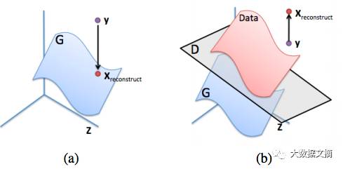
(a): Ideal reconstruction of y from the generative distribution (blue surface). (b): A failed attempt to reconstruct y by maximizing D(y). Image from the image repair paper.

2. [ML-Heavy] Loss Function for Projection to pgpg

To give a reasonable definition for the projection, we first define some symbols for image inpainting. We use a binary mask M (mask), which only has values of 0 and 1. A value of 1 indicates the part of the image we want to keep, while a value of 0 indicates the part we need to fill in. Now we can define how to inpaint y given the binary mask M. The elements in y are multiplied by the elements in M. The element-wise multiplication of the two matrices is also called the Hadamard product, represented as M⊙y. M⊙y represents the original part of the image.

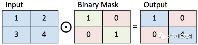
Binary mask illustration

Next, suppose we have found a z^, which can generate a reasonable reconstruction of the missing values with G(z^). The pixels to be filled in (1−M)⊙G(z^) can be added to the original pixels to obtain the reconstructed image:

x_reconstructed = M⊙y + (1−M)⊙G(z^)

Now what we need to do is find a suitable G(z^) for image inpainting. To find z^, we revisit the contextual and perceptual losses mentioned at the beginning of the article and use them as the context for DCGANs. For this, we define a loss function for any z∼pz.

The smaller the loss function, the more suitable z^ is.

Contextual loss: To obtain the same context as the input image, we need to ensure that the G(z) corresponding to the known pixels in y is as similar as possible. Therefore, when the output of G(z) is not similar to the known pixel locations in y, we need to penalize G(z). For this, we subtract G(z) from the pixels in y at the corresponding positions and obtain the degree of dissimilarity:

L_contextual(z) = ||M⊙G(z) − M⊙y||

where ||x||1 = ∑i |xi| is the l1 norm of some vector x. The l2 norm is also acceptable, but the paper states that practice shows that the l1 norm performs better.

Ideally, the pixels of y and G(z) for the known positions are equal. That is, for the known pixel positions i, ||M⊙G(z)i − M⊙yi|| = 0, L_contextual(z) = 0.

Perceptual loss: To reconstruct a visually realistic image, we need to ensure that the discriminator determines that the image looks real. To achieve this, we perform the same steps as in training the DCGAN.

L_perceptual(z) = log(1−D(G(z)))

Finally, by combining the contextual loss and perceptual loss, we can find z^:

L(z) = L_contextual(z) + λL_perceptual(z) z^ = argmin_z L(z)

where λ is a hyperparameter that controls the importance of contextual loss relative to perceptual loss. (I used the default λ=0.1 and did not study this value in depth.) Then, as mentioned earlier, we use G(z) to reconstruct the missing parts in y.

L_contextual(z) = ||M⊙G(z) − M⊙y||

The image also uses Poisson blending to smooth the image.

3. [ML-Heavy] Using TensorFlow for DCGAN Image Inpainting

This chapter provides my modifications to Taehoon Kim’s carpedm20/DCGAN-tensorflow code for image inpainting.

self.mask = tf.placeholder(tf.float32, [None] + self.image_shape, name=’mask’)

By performing gradient descent on the gradient ∇zL(z), we can iteratively find argmin_z L(z). After defining the loss function, TensorFlow’s automatic differentiation can automatically compute this value for us! Therefore, the complete implementation based on DCGANs can be achieved by adding four lines of TensorFlow code to the existing DCGAN implementation. (Of course, implementing it also requires some non-TensorFlow code.)

self.contextual_loss = tf.reduce_sum(

tf.contrib.layers.flatten(

tf.abs(tf.mul(self.mask, self.G) – tf.mul(self.mask, self.images))), 1)

self.perceptual_loss = self.g_loss

self.complete_loss = self.contextual_loss + self.lam * self.perceptual_loss

self.grad_complete_loss = tf.gradients(self.complete_loss, self.z)

Next, we define the mask. I only added one in the central area of the image; you can add others, like random masks, and then submit a pull request.

if config.maskType == ‘center’:

scale = 0.25

assert(scale <= 0.5)

mask = np.ones(self.image_shape)

l = int(self.image_size * scale)

u = int(self.image_size * (1.0 – scale))

mask[l:u, l:u, :] = 0.0

For the gradient descent, we use mini-batch, momentum-based projected gradient descent for z in [-1, 1].

for idx in xrange(0, batch_idxs):

batch_images = …

batch_mask = np.resize(mask, [self.batch_size] + self.image_shape)

zhats = np.random.uniform(-1, 1, size=(self.batch_size, self.z_dim))

v = 0

for i in xrange(config.nIter):

fd = {

self.z: zhats,

self.mask: batch_mask,

self.images: batch_images,

}

run = [self.complete_loss, self.grad_complete_loss, self.G]

loss, g, G_imgs = self.sess.run(run, feed_dict=fd)

v_prev = np.copy(v)

v = config.momentum * v – config.lr * g[0]

zhats += -config.momentum * v_prev + (1 + config.momentum) * v

zhats = np.clip(zhats, -1, 1)

4. Filling in Images

Select some images for inpainting and place them in dcgan-completion.tensorflow/your-test-data/raw. Then arrange them neatly as in dcgan-completion.tensorflow/your-test-data/aligned. Here I randomly selected some images from LFW. My DCGAN did not use images from LFW for training.

You can fill in images like this:

./complete.py ./data/your-test-data/aligned/* –outDir outputImages

This code will generate images and periodically output them in the –outDir folder. You can use ImageMagick to create a gif:

cd outputImages

convert -delay 10 -loop 0 completed/*.png completion.gif

Final image inpainting. The center of the image is generated automatically. The source code can be downloaded from here. This is a sample I randomly selected from LFW.

Thank you for reading, and we have succeeded! In this article, we covered a method for image inpainting:

1. Understanding images as distributions of probabilities. 2. Generating pseudo-images. 3. Finding the best pseudo-images for filling in.

My example is for faces, but DCGANs can also be used on other types of images. Overall, GANs are challenging to train, and we are still unclear on how to train them for specific types of objects and how to train on large images. However, this is a promising model, and I look forward to what GANs will create for us in the future!

👇 Click to read the original text, fill out the questionnaire, and get rewards

Original text: http://bamos.github.io/2016/08/09/deep-completion/?utm_source=mybridge&utm_medium=blog&utm_campaign=read_more

About Reposting

If you need to repost, please indicate the author and source prominently at the beginning of the article (transferred from: Big Data Digest | bigdatadigest), and place a prominent QR code for Big Data Digest at the end of the article. Articles without original markings can be directly reposted according to reposting requirements; please send the repost link to us after reposting; for articles with original markings, please send [Article Name - Awaiting Authorization Public Account Name and ID] to us to apply for whitelist authorization. Unauthorized reposting and adaptation will be subject to legal liability. Contact email: [email protected].