This article introduces the basic concepts in deep learning neural networks:
-
Vectors, Matrices, and Multidimensional Arrays -
Basics of Neural Networks -
Activation Functions -
Implementing Fully Connected Networks from Scratch
Mathematics and Python Basics
In neural networks, vectors and matrices are ubiquitous. Below is an introduction to creating one-dimensional, two-dimensional, and higher-dimensional arrays using numpy.
Vector (One-Dimensional Array)
A vector is a quantity that has both magnitude and direction, and it can be represented as a collection of numbers arranged in a row.
In [1]:
<span>import numpy as np</span>In [2]:
<span><span># Create a row vector </span>row_vector = np.array([1, 2, 3, 4, 5]) <span>print</span>(<span>"Row Vector: "</span>) <span>print</span>(row_vector) Row Vector: [1 2 3 4 5]</span>In [3]:
<span><span># Create a column vector </span>col_vector = np.array([[1], [2], [3],[4],[5]]) <span>print</span>(<span>"Column Vector: "</span>) <span>print</span>(col_vector)Column Vector: [[1] [2] [3] [4] [5]]</span>Matrix (Two-Dimensional Array)
Create a 3×3 matrix:
In [4]:
<span><span># Create a 3x3 matrix</span>matrix = np.array([[1, 2, 3], [4, 5, 6], [7, 8, 9]])<span>print</span>(<span>"Original Matrix: "</span>)<span>print</span>(matrix)Original Matrix: [[1 2 3] [4 5 6] [7 8 9]]</span>Operations related to matrices:
In [5]:
<span><span># 1- Calculate the transpose of the matrix</span>transpose_matrix = np.transpose(matrix)<span>print</span>(<span>"Transpose Matrix: "</span>)<span>print</span>(transpose_matrix)Transpose Matrix: [[1 4 7] [2 5 8] [3 6 9]]</span>You can also use the T property of the matrix to achieve transposition:
In [6]:
<span>matrix.T</span>Out[6]:
<span>array([[1, 4, 7], [2, 5, 8], [3, 6, 9]])</span>Next, we introduce how to find the inverse of a matrix (only square matrices have inverses):
Given a matrix A, if E is the identity matrix, then matrix B is called the inverse matrix of matrix A.
Not all square matrices have an inverse; when a square matrix is non-invertible, the concept of the zero matrix is introduced.
In [7]:
<span><span># 2- Calculate the inverse of the matrix</span>inverse_matrix = np.linalg.inv(matrix)<span>print</span>(<span>"Inverse Matrix: "</span>)<span>print</span>(inverse_matrix)Inverse Matrix: [[ 3.15251974e+15 -6.30503948e+15 3.15251974e+15] [-6.30503948e+15 1.26100790e+16 -6.30503948e+15] [ 3.15251974e+15 -6.30503948e+15 3.15251974e+15]]</span>The determinant of matrix A is represented as |A| or det(A): If the determinant of a matrix is not zero, then the matrix is invertible; conversely, if the determinant is zero, it is non-invertible.
In [8]:
<span><span># Calculate the determinant of the matrix</span>determinant = np.linalg.det(matrix)<span>print</span>(<span>"Determinant: "</span>)<span>print</span>(determinant)Determinant: -9.51619735392994e-16</span>Multidimensional Arrays
Extending vectors and matrices to N dimensions results in multidimensional arrays.
1. Create a tensor of all zeros:
In [9]:
<span>tensor = np.zeros((2, 3, 4, 4))tensor</span>Out[9]:
<span>array([[[[0., 0., 0., 0.], [0., 0., 0., 0.], [0., 0., 0., 0.], [0., 0., 0., 0.]], [[0., 0., 0., 0.], [0., 0., 0., 0.], [0., 0., 0., 0.], [0., 0., 0., 0.]], [[0., 0., 0., 0.], [0., 0., 0., 0.], [0., 0., 0., 0.], [0., 0., 0., 0.]]], [[[0., 0., 0., 0.], [0., 0., 0., 0.], [0., 0., 0., 0.], [0., 0., 0., 0.]], [[0., 0., 0., 0.], [0., 0., 0., 0.], [0., 0., 0., 0.], [0., 0., 0., 0.]], [[0., 0., 0., 0.], [0., 0., 0., 0.], [0., 0., 0., 0.], [0., 0., 0., 0.]]]])</span>In [10]:
<span>tensor.shape <span># Shape of the multidimensional array</span></span>Out[10]:
<span>(2, 3, 4, 4)</span>In [11]:
<span>tensor.size <span># Total number of elements in the array</span></span>Out[11]:
<span>96</span>In [12]:
<span>tensor.ndim <span># Represents 4 dimensions</span></span>Out[12]:
<span>4</span>2. Create an array of all ones
In [13]:
<span>tensor1 = np.ones((2,4,3))tensor1</span>Out[13]:
<span>array([[[1., 1., 1.], [1., 1., 1.], [1., 1., 1.], [1., 1., 1.]], [[1., 1., 1.], [1., 1., 1.], [1., 1., 1.], [1., 1., 1.]]])</span>In [14]:
<span>tensor1.ndim <span># Represents 3 dimensions</span></span>Out[14]:
<span>3</span>3. Create a custom array
In [15]:
<span>tensor2 = np.arange(48)tensor2</span>Out[15]:
<span>array([ 0, 1, 2, 3, 4, 5, 6, 7, 8, 9, 10, 11, 12, 13, 14, 15, 16, 17, 18, 19, 20, 21, 22, 23, 24, 25, 26, 27, 28, 29, 30, 31, 32, 33, 34, 35, 36, 37, 38, 39, 40, 41, 42, 43, 44, 45, 46, 47])</span>In [16]:
<span>tensor2.ndim</span>Out[16]:
<span>1</span>Change the shape implementation:
In [17]:
<span>tensor2.reshape((2,8,3))</span>Out[17]:
<span>array([[[ 0, 1, 2], [ 3, 4, 5], [ 6, 7, 8], [ 9, 10, 11], [12, 13, 14], [15, 16, 17], [18, 19, 20], [21, 22, 23]], [[24, 25, 26], [27, 28, 29], [30, 31, 32], [33, 34, 35], [36, 37, 38], [39, 40, 41], [42, 43, 44], [45, 46, 47]]])</span>In [18]:
<span><span># The effect is the same: numpy will automatically infer the value of -1 in the dimension</span>tensor2.reshape((2,8,-1))</span>Out[18]:
<span>array([[[ 0, 1, 2], [ 3, 4, 5], [ 6, 7, 8], [ 9, 10, 11], [12, 13, 14], [15, 16, 17], [18, 19, 20], [21, 22, 23]], [[24, 25, 26], [27, 28, 29], [30, 31, 32], [33, 34, 35], [36, 37, 38], [39, 40, 41], [42, 43, 44], [45, 46, 47]]])</span>NumPy Broadcasting Mechanism
In NumPy multidimensional arrays, arrays with different shapes can also perform operations. See the example below:
In [19]:
<span>A = np.array([[1,2,3], [4,5,6]])A</span>Out[19]:
<span>array([[1, 2, 3], [4, 5, 6]])</span>In [20]:
<span>A * 100</span>Out[20]:
<span>array([[100, 200, 300], [400, 500, 600]])</span>This is equivalent to multiplying 100 by [[100,100,100],[100,100,100]] and then multiplying it with the corresponding elements in array A.
In [21]:
<span>A + 200</span>Out[21]:
<span>array([[201, 202, 203], [204, 205, 206]])</span>Broadcasting mechanism in addition:
In [22]:
<span>A + [100,200,300]</span>Out[22]:
<span>array([[101, 202, 303], [104, 205, 306]])</span>Dot Product
The inner product of vectors is a specific numerical value:
In [23]:
<span>a = np.array([1,2,3])b = np.array([4,5,6])</span>In [24]:
<span>a * b <span># Matrix multiplication</span></span>Out[24]:
<span>array([ 4, 10, 18])</span>In [25]:
<span>np.dot(a,b) <span># 4+10+18=32</span></span>Out[25]:
<span>32</span>In [26]:
<span>sum(a * b) <span># The result of matrix multiplication is the product</span></span>Out[26]:
<span>32</span>Inner product of matrices:
In [27]:
<span>c = np.array([[1,2],[3,4]])d = np.array([[5,6],[7,8]])</span>In [28]:
<span>c</span>Out[28]:
<span>array([[1, 2], [3, 4]])</span>In [29]:
<span>d</span>Out[29]:
<span>array([[5, 6], [7, 8]])</span>In [30]:
<span>np.dot(c,d)</span>Out[30]:
<span>array([[19, 22], [43, 50]])</span>-
15+27=19 -
16+28=22 -
35+47=43 -
36+48=50
Basics of Neural Networks
Basic Principles
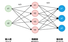
A neural network is a complex function. A function is a transformer that converts certain inputs into certain outputs, and the function of a neural network is similar:
Denote the data of the input layer, represents the weights, and represents the bias.
The result of the first hidden neuron can be expressed as:
The neurons in the hidden layer are calculated based on the weighted sum.
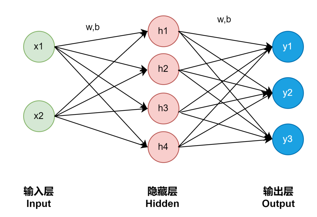
-
The basic neural network has three layers: input layer, hidden layer, and output layer.
-
The arrows carry two pieces of information: weight w and bias b; the weight is multiplied by the value of the neuron and then added to the bias, and the resulting value after passing through an activation function is used as the input to the next neuron.
Implementation of the Hidden Layer
A network where all adjacent neurons are connected through weights and biases is also called a fully connected network.
The complete calculations based on the matrix product for four hidden neurons:
It can be abbreviated as:
Where is 1×2, is 2×4, and is 1×4.
Now let’s implement the calculations for the hidden layer:
In [31]:
<span><span># Simple implementation of hidden layer calculations</span>W1 = np.random.randn(2,4)b1 = np.random.randn(4) <span># Broadcasting mechanism will occur</span>x = np.random.randn(10,2)h = np.dot(x,W1) + b1h</span>Out[31]:
<span>array([[-0.80051904, -0.98416179, 1.7341734 , -2.04167071], [ 0.78748052, 1.16324088, 1.06046707, -0.14729655], [ 0.48977828, 1.97419074, -0.2551278 , -1.81056956], [-1.70298304, -1.89547071, 1.74981458, -3.45140937], [-0.33747008, 0.19029478, 0.88625396, -2.08032192], [-0.83369394, -0.94217107, 1.64505112, -2.17486955], [ 1.76349184, 3.52267844, -0.58885411, -0.10364203], [ 0.68911993, 1.36470324, 0.70478019, -0.62518316], [ 2.28604672, 5.22576684, -1.99452197, -0.55441134], [ 1.67011023, 1.98066418, 1.13292561, 1.31107412]])</span>Activation Functions
The transformation of the fully connected layer network is a linear transformation. Using activation functions can give it a “non-linear” effect. Using activation functions can enhance the expressiveness of the neural network.
Here are some commonly used activation functions:
1. Sigmoid Function
In [32]:
<span>import numpy as npimport matplotlib.pyplot as plt<span># Define function</span>def sigmoid(x): <span>return</span> 1 / (1 + np.exp(-x))<span># x-y</span>x = np.linspace(-10, 10, 100)y = sigmoid(x)plt.plot(x, y)plt.xlabel(<span>'x'</span>)plt.ylabel(<span>'sigmoid(x)'</span>)plt.title(<span>'Sigmoid Function'</span>)plt.grid(True)plt.show()</span>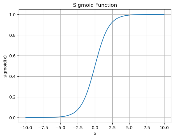
2. ReLU Activation Function:
In [33]:
<span>import numpy as npimport matplotlib.pyplot as pltdef relu(x): <span>return</span> np.maximum(0, x)x = np.linspace(-10, 10, 100)y = relu(x)plt.plot(x, y)plt.xlabel(<span>'x'</span>)plt.ylabel(<span>'ReLU(x)'</span>)plt.title(<span>'ReLU Function'</span>)plt.grid(True)plt.show()</span>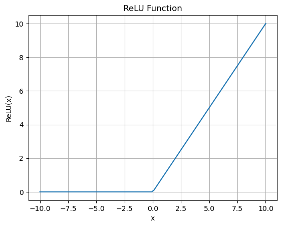
3. Tanh Function:
In [34]:
<span>import numpy as npimport matplotlib.pyplot as plt<span># Define Tanh function</span>def tanh(x): <span>return</span> np.tanh(x)<span># Generate x values</span>x = np.linspace(-10, 10, 1000)<span># Calculate y values</span>y = tanh(x)<span># Plot image</span>plt.plot(x,y)plt.xlabel(<span>'x'</span>)plt.ylabel(<span>'tanh(x)'</span>)plt.title(<span>'Tanh Function'</span>)plt.grid(True)plt.show()</span>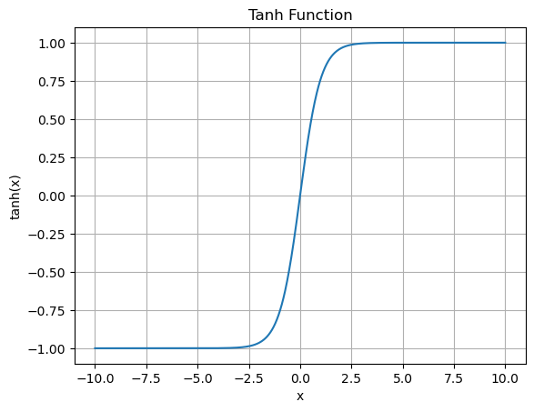
Neural Network with Sigmoid Activation Function
In [35]:
<span>def sigmoid(x):    <span>"""    Define sigmoid function    """    <span>return</span> 1 / (1 + np.exp(-x))x = np.random.randn(10,2)W1 = np.random.randn(2,4)b1 = np.random.randn(4)W2 = np.random.randn(4,3)b2 = np.random.randn(3)<span>print</span>(<span>"W1:

"</span>,W1)<span>print</span>(<span>"b1:

"</span>,b1)<span>print</span>(<span>"W1:

"</span>,W2)<span>print</span>(<span>"b1:

"</span>,b2)W1: [[-0.81716844 -0.2700162   0.47712972  1.52610728] [-0.13728734 -0.48808859 -0.39338065  0.75255599]]b1: [ 1.21057066  0.14936438  0.8861704  -0.49434345]W1: [[ 0.77540225 -0.0813373   1.61562571] [ 0.18555707 -1.57503291 -1.48010281] [-1.26013418 -0.71906974  1.98427043] [-0.09948728 -0.06870956 -0.0222825 ]]b1: [ 1.24730692 -0.26517252 -0.21867687]</span></span>
In the example above, there are 10 sample data points: , corresponding to 10 hidden layer neurons
In [36]:
<span>h = np.dot(x,W1) + b1 <span># Hidden neurons</span>a = sigmoid(h) <span># Use activation function on hidden neurons</span>a</span>Out[36]:
<span>array([[0.89036829, 0.68166094, 0.6709089 , 0.07559634], [0.61832049, 0.42523258, 0.74774176, 0.75044002], [0.34969505, 0.34159362, 0.85077636, 0.95890215], [0.80167595, 0.4228318 , 0.55454109, 0.43608519], [0.7444589 , 0.34582381, 0.54414278, 0.64542647], [0.86841737, 0.75140648, 0.78167754, 0.07047421], [0.73173076, 0.58966053, 0.78724036, 0.39576964], [0.95512889, 0.64006136, 0.40382409, 0.02324403], [0.5662982 , 0.40702709, 0.77004949, 0.81874147], [0.46174302, 0.57379292, 0.91075142, 0.79929614]])</span>In [37]:
<span>s = np.dot(a,W2) + b2 <span># Output neurons</span>s</span>Out[37]:
<span>array([[ 1.21123139, -1.89885556, 1.54047697], [ 0.78874474, -1.57446122, 1.61790986], [ 0.41435542, -1.50929024, 1.50750941], [ 1.20520658, -1.42506962, 1.54133929], [ 1.13882744, -1.30603225, 1.53757998], [ 1.06807862, -2.0862201 , 1.62169098], [ 0.89270575, -1.84669814, 1.64404699], [ 1.5954989 , -1.64295259, 1.17787556], [ 0.71012253, -1.5622894 , 1.60354995], [ 0.48462603, -1.91628525, 1.46742132]])</span>Using another fully connected layer to transform the output of this activation function.
The hidden layer has four neurons, and the output layer has three neurons, so the shape of the weight matrix used in the fully connected layer is set to.
Complete Code
The complete code for the entire process is:
In [38]:
<span><span># Complete code for neural network + sigmoid activation function</span>import numpy as npdef sigmoid(x): <span>return</span> 1 / (1+np.exp(-x))x = np.random.randn(10,2) <span># 10*2</span>W1 = np.random.randn(2, 4) <span># 2*4 # 4 represents the number of hidden neurons; 2 matches the input x's x.shape[1]</span>b1 = np.random.randn(4) <span># 10*4; the bias must be 4</span>W2 = np.random.randn(4, 3) <span># 4*3 # 3 represents the number of output neurons; 4 is the shape[1] of the first hidden neurons</span>b2 = np.random.randn(3) <span># 10*3; the bias must be 3</span>h = np.dot(x, W1) + b1a = sigmoid(h)s = np.dot(a, W2) + b2s</span>Out[38]:
<span>array([[ 1.52757614, -1.50378018, 0.69751311], [ 2.16511559, -1.24918194, 0.23662412], [ 2.76594566, -1.29153453, -0.57892373], [ 2.41784231, -1.19402867, 0.22564103], [ 1.26703665, -1.46154016, 1.37571233], [ 2.15837849, -1.33121603, 0.69843425], [ 2.02575248, -1.32591319, 0.9561904 ], [ 2.02329408, -1.30629759, 0.93633673], [ 2.24129269, -1.22068445, 0.50451103], [ 2.74841634, -1.30657481, -0.51901695]])</span>Implementation of Neural Network Layers (Classes)
Forward Propagation
Forward propagation refers to the process in which information in a neural network starts from the input layer, is processed by the neurons in each layer, and finally reaches the output layer.
During forward propagation, each layer’s neurons take the output of the previous layer as input, and after internal calculations, pass the results to the next layer. This process continues until the output layer, producing the final output of the network.
During forward propagation, the input and output of neurons are connected through weights, and undergo non-linear transformations through activation functions, allowing the network to learn and simulate complex non-linear relationships.
Backward Propagation
Backward propagation is an optimization algorithm used to train neural networks.
It updates parameters by calculating the gradient of the loss function with respect to the neural network parameters, thereby minimizing the loss function. During the training process of the neural network, the backward propagation algorithm adjusts the weights of each node by backpropagating the output error of each node, enabling the network to predict results more accurately.
Specifically, a set of training data is first input into the network, and the output result is calculated. Then the difference between the output result and the actual result, which is the network’s error, is calculated. Next, the contribution of each node to the error is calculated, and these contributions are backpropagated to the previous layer. Based on the size of the contributions, the weights of each node are adjusted to reduce the error. This process is repeated until the error reaches a certain level. By continuously adjusting the weights, the backward propagation algorithm can make the network predict results more accurately.
Defining Network Layers
-
The transformation of the sigmoid activation function: Sigmoid Layer -
The transformation of the fully connected layer is equivalent to a geometric field of affine transformation: Affine Layer
Code conventions:
-
All layers use the forward() and backward() methods, representing forward and backward propagation, respectively. -
All layers use params and grads instance variables; where params is a list that stores weight and bias parameters (which may have multiple parameters, using a list), and grads corresponds to the parameters in params.
Sigmoid Layer
Defining the Sigmoid layer for the activation function:
In [39]:
<span>import numpy as npclass Sigmoid: def __init__(self): self.params = [] <span># No learnable parameters, using an empty list</span> def forward(self,x): <span>return</span> 1 / (1 + np.exp(-x))</span>Affine Layer
Defining the Affine layer for fully connected layers:
In [40]:
<span>class Affine: def __init__(self, W, b): <span>""" Initialize parameters: weights W and biases b """</span> self.params = [W,b] <span># Parameter list saves: W-weight b-bias</span> def forward(self, x): <span>""" Forward propagation function based on matrix dot product """</span> W,b = self.params <span># Assign parameters from the list to W and b</span> out = np.dot(x,W) + b <span># Implement forward propagation function</span> <span>return</span> out</span>TwoLayerNet Network
In [41]:
<span>class TwoLayerNet: def __init__(self, input_size, hidden_size, output_size): <span>""" Initialize method: number of neurons in input layer - number of neurons in hidden layer - number of neurons in output layer """</span> I,H,O = input_size, hidden_size, output_size <span># Connect input layer and hidden layer</span> W1 = np.random.randn(I,H) <span># Initial values for weights and biases</span> b1 = np.random.randn(H) <span># Connect hidden layer and output layer</span> W2 = np.random.randn(H,O) b2 = np.random.randn(O) <span># Define a list of layers, containing fully connected layer 1, activation layer, fully connected layer 2</span> self.layers = [ Affine(W1, b1), Sigmoid(), Affine(W2,b2) ] <span># Gather all weights into a list</span> self.params = [] <span>for</span> layer <span>in</span> self.layers: <span># Loop through each layer</span> self.params += layer.params <span># Weight parameters are placed in the params list </span> def predict(self, x): <span>for</span> layer <span>in</span> self.layers: x = layer.forward(x) <span># Use the forward update method for each layer, ultimately outputting Out</span> <span>return</span> x</span>Defining a class named <span>TwoLayerNet</span> representing a neural network with two hidden layers. Below is a detailed explanation of the code:
-
Initialization Method (
<span>__init__</span>):
-
The first layer: a linear transformation layer (implemented through <span>Affine</span>) connecting the input layer and hidden layer. -
The second layer: a Sigmoid activation function layer (implemented through <span>Sigmoid</span>). -
The third layer: a linear transformation layer (implemented through <span>Affine</span>) connecting the hidden layer and output layer.
-
<span>input_size</span>: The number of neurons in the input layer. -
<span>hidden_size</span>: The number of neurons in the hidden layer. -
<span>output_size</span>: The number of neurons in the output layer. -
Input parameters:
-
<span>W1</span>and<span>b1</span>: Randomly generated weights matrix and bias for connecting the input layer and hidden layer. -
<span>W2</span>and<span>b2</span>: Randomly generated weights matrix and bias for connecting the hidden layer and output layer.self.layers: Defines a list of layers containing the following three layers:
-
<span>self.params</span>: Used to store all weight parameters.
Prediction Method (<span>predict</span>):
-
Input parameter: <span>x</span>: Input data. -
For each layer, use its <span>forward</span>method for forward propagation, updating the value of<span>x</span>. -
Finally, return the updated <span>x</span>value. This is usually the output of the network.
The network does not include the update process for the bias terms, so the bias terms are only used in forward propagation and are not updated in backward propagation.
Forward Propagation Example
In [42]:
<span>x = np.random.randn(10,2)model = TwoLayerNet(2,4,3)s = model.predict(x)s</span>Out[42]:
<span>array([[-0.11149934, 2.92086863, 0.02600311], [-0.52853339, 2.55687161, 0.09639072], [-0.37599196, 2.70311037, 0.07967748], [-0.08386817, 2.84851586, 0.09121393], [-0.36363321, 2.50668478, 0.14880286], [-0.18938764, 2.80382617, 0.08435871], [-0.36065023, 2.69994522, 0.08593762], [-0.38339136, 2.57659206, 0.12620684], [-0.29318787, 2.68147118, 0.1135041 ], [ 0.15702997, 2.94857814, 0.09733163]])</span>Learning in Neural Networks
The process of neural networks is generally to learn first, and then use the good parameters for inference. To know how effective the learning is, an indicator is usually needed. This indicator is generally referred to as loss.
Loss Function (Softmax)
Based on supervised learning or the prediction results of neural networks, the degree of difference from the actual results is calculated. This means calculating the scalar value of the model’s poor performance, which is the loss.
In multi-class classification problems, the commonly used loss function is <span>cross entropy</span>.
Drawing the softmax function curve:
In [43]:
<span>import numpy as npimport matplotlib.pyplot as pltdef softmax(x): e_x = np.exp(x - np.max(x)) <span>return</span> e_x / e_x.sum()<span># Generate input data</span>x = np.linspace(-10, 10, 100)<span># Calculate softmax values</span>y = softmax(x)<span># Draw softmax curve</span>plt.plot(x, y)plt.xlabel(<span>'x'</span>)plt.ylabel(<span>'softmax(x)'</span>)plt.title(<span>'Softmax Function'</span>)plt.grid(True)plt.show()</span>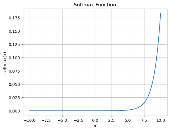
The elements output by the Softmax function are real numbers between 0.0 and 1.0. If all these elements are summed, the total equals 1. Therefore, the output of Softmax can be interpreted as probabilities. This probability is then input into the cross-entropy error. The cross-entropy error is represented as:
-
Corresponding to the k-th category of supervised labels -
log is the logarithm with base e
Considering mini-batch processing, the cross-entropy error can be expressed as:
Assuming there are N data points, represents the value of the k-th dimension element of the n-th data; represents the output of the neural network, and represents the supervised label.
Derivatives and Gradients
Derivatives
The goal of learning in neural networks is to find a combination of parameters that minimizes the loss. A brief introduction to derivatives and gradients:
For a function, the derivative of L with respect to x is denoted as , representing the degree of change. Specifically, how much a small change in x will cause L to change.
The derivative with respect to can be expressed as:
Gradient
Thus, the derivative for all x is:
Listing the derivatives of L with respect to each element of the vector gives the gradient gradient.
Matrix solving for gradients:
Where is the matrix, and
have the same shape.
Chain Rule
During the learning phase, the neural network outputs loss after the given learning data. Once we have the gradients of the loss with respect to each parameter, we can use these gradients to update the parameters.
How to find the gradients of the neural network? Using the backward propagation method. The key to understanding the backward propagation method is the chain rule. The chain rule is the derivative rule for composite functions, where composite functions are functions composed of multiple functions.
Consider two functions: and , then: , so the derivative of z with respect to x is:
MatMul Layer Implementation
Implementing the layer for matrix operations:
In [44]:
<span>class MatMul: def __init__(self, W): self.params = [W] <span># Save the learnable parameter, only weight W at this time</span> self.grads = [np.zeros_like(W)] <span># Gradients are stored in grads</span> self.x = None <span># Forward propagation</span> def forward(self, x): W, = self.params <span># Parameters</span> out = np.dot(x,W) <span># Output</span> self.x = x <span>return</span> out <span># Backward propagation</span> def backword(self, dout): W, = self.params dx = np.dot(dout, W.T) dW = np.dot(self.x.T, dout) <span># grads[0][...] uses ellipsis: can fix the memory address of the Numpy array and overwrite the elements of the Numpy array</span> <span># grads[0]=dW shallow copy grads[0][...] = dW deep copy</span> self.grads[0][...] = dW <span># Set the gradient of the weights in the instance variable grads; each element in the grads list is a Numpy array</span> <span>return</span> dx</span>About Numpy’s […] Copy Issue
Example
This actually discusses the issue of shallow and deep copies.
In [45]:
<span>a = np.array([1, 2, 3])b = np.array([4, 5, 6])</span>In [46]:
<span><span>print</span>(<span>"Original data a's address: "</span>, id(a))<span>print</span>(<span>"Original data b's address: "</span>, id(b))Original data a's address: 2575053791920Original data b's address: 2575053167312</span>In [47]:
<span>a = b <span># Assign b to a;</span>a</span>Out[47]:
<span>array([4, 5, 6])</span>Check the memory addresses of a and b again:
In [48]:
<span><span>print</span>(<span>"After a=b, data a's address: "</span>, id(a))<span>print</span>(<span>"After a=b, data b's address: "</span>, id(b)) After a=b, data a's address: 2575053167312After a=b, data b's address: 2575053167312</span>It can be seen that a and b’s memory addresses are exactly the same. This means that a’s reference is assigned to b, and now a and b point to the same memory location.
In [49]:
<span>a = np.array([1, 2, 3])b = np.array([4, 5, 6]) </span>In [50]:
<span><span>print</span>(<span>"Original data a's address: "</span>, id(a))<span>print</span>(<span>"Original data b's address: "</span>, id(b))Original data a's address: 2575054711248Original data b's address: 2575054715760</span>In [51]:
<span>a[...] = b <span># Assignment</span></span>In [52]:
<span><span>print</span>(<span>"After a[...]=b, data a's address: "</span>, id(a))<span>print</span>(<span>"After a[...]=b, data b's address: "</span>, id(b)) After a[...]=b, data a's address: 2575054711248After a[...]=b, data b's address: 2575054715760</span>It can be seen that a and b’s memory addresses are different; and a’s address is still the same as before the assignment.
<span>a[...] = b</span>indicates an in-place modification of the data: it is currently assigning array b to array a, because this is an in-place operation, a and b still point to the same memory address.
Conclusion
In the above example, <span>a = b</span> is a shallow copy, while <span>a[...] = b</span> is a deep copy.
-
<span>a = b</span>is a shallow copy because it creates a new reference a that points to the same memory address as b. At this point, modifying the value of b will also affect a since they reference the same object. -
<span>a[...] = b</span>is a deep copy because it modifies the values of array a in place, making it equal to array b. This operation does not affect the memory address of array b, but just copies the values of b into a. Therefore, even if b’s values are modified later, it will not affect a’s values.
Gradient Derivation and Backward Propagation Implementation
Sigmoid Layer
Implementing the forward and backward processes based on the Sigmoid function:
In [53]:
<span>class Sigmoid: def __init__(self): self.params, self.grads = [], [] <span># Save parameters and their gradients</span> self.out = None <span># Store the result of forward propagation </span> def forward(self, x): <span># Forward propagation process; output through Sigmoid function</span> out = 1 / (1 + np.exp(-x)) <span># sigmoid function</span> self.out = out <span># Save output out</span> <span>return</span> out def backward(self, dout): <span># Backward propagation process</span> dx = dout * (1.0 - self.out) * self.out <span># The derivative of sigmoid is y*(1-y)</span> <span>return</span> dx <span># Return gradient</span></span>Affine Layer
Through the implementation of the Affine layer’s forward propagation.
In [54]:
<span>class Affine: def __init__(self, W, b): <span>""" Class initialization function, accepts two parameters """</span> <span># Save weights matrix and bias vector</span> self.params = [W,b] <span># Initialize two zero gradient arrays, with shapes the same as the weights matrix and bias vector, stored in the instance's grads attribute</span> self.grads = [np.zeros_like(W), np.zeros_like(W)] self.x = None def forward(self, x): <span>""" Define forward propagation method """</span> W,b = self.params <span># Extract weights and biases from params attribute</span> out = np.dot(x,W) + b <span># Forward output: based on linear transformation</span> self.x = x <span># Save input x in the instance's x attribute</span> <span>return</span> out def backword(self, dout): <span>""" Define backward propagation method """</span> W, b = self.params <span># Extract weights and biases from params attribute</span> dx = np.dot(dout, W.T) <span># Calculate gradients through dot product</span> dW = np.dot(self.x.T, dout) <span># Calculate gradients with respect to the weights matrix</span> db = np.sum(dout, axis=0) <span># Calculate gradients with respect to the bias vector</span> self.grads[0][...] = dW <span># Store weights and gradients in the instance's grads attribute</span> self.grads[1][...] = db <span>return</span> dx</span>Weight Updates
After obtaining the gradients through the error backpropagation method, the parameters of the neural network can be updated using these gradients.
Step 1: Mini-batch
-
Randomly select multiple data points from the training data
Step 2: Calculate gradients
-
Based on error backpropagation, calculate the gradients of the loss function with respect to each weight parameter
Step 3: Update parameters
-
Use gradients to update weight parameters
Repeat Steps 1-2-3
The gradients mentioned here point to the direction in which the loss increases the most at the current weight parameters. Typically, the parameters are updated in the opposite direction of this gradient to accelerate the reduction of loss, which is called gradient descent.
Next, we introduce Stochastic Gradient Descent (SGD). Stochastic refers to the gradient of the selected data (mini-batch).
Where represents the learning rate, e.g., 0.001, 0.01, etc.
In [55]:
<span>class SGD: def __init__(self, lr=0.01): self.lr = lr <span># Set learning rate</span> def update(self, params, grads): <span>for</span> i <span>in</span> range(len(params)): params[i] -= self.lr * grads[i] <span># Update parameters</span></span>Using the SGD class to update the parameters of the neural network (providing pseudocode)
<span><span># Pseudocode</span>model = TwoLayerNet(...)optimizer = SGD()<span>for</span> i <span>in</span> range(10000): x_batch, t_batch = get_mini_batch() loss = model.farward(x_batch, t_batch) model.backward() optimizer.update(model.params, model.grads)</span>
END