Image Classification with Few-Shot Learning Using PyTorch

In recent years, deep learning-based models have performed excellently in tasks such as object detection and image recognition. Challenging image classification datasets like ImageNet, which contains 1000 different object categories, have seen some models surpass human-level performance. However, these models rely on supervised training processes, and the availability of labeled training data significantly impacts them. Moreover, the categories that the models can detect are limited to the classes they have been trained on.

Due to insufficient labeled images for all classes during training, these models may be less useful in real-world environments. We desire models that can recognize classes they have not seen during training, as it is almost impossible to train on images of all potential objects. The problem of learning from just a few samples is called “Few-Shot Learning.”

What is Few-Shot Learning?

Few-Shot Learning is a subfield of machine learning. It involves classifying new data with only a few training samples and supervisory data. With just a small number of training samples, the models we create can perform quite well.

Consider the following scenario: In the medical field, there may not be enough X-ray images for training for some rare diseases. In such scenarios, building a few-shot learning classifier is the perfect solution.

Types of Few-Shot Learning

Generally, researchers have identified four types:

1. N-Shot Learning (NSL)

2. Few-Shot Learning (FSL)

3. One-Shot Learning (OSL)

4. Zero-Shot Learning (ZSL)

When we talk about FSL, we usually refer to N-way-K-Shot classification. N represents the number of classes, and K represents the number of samples to train for each class. Thus, N-Shot Learning is regarded as a broader concept than all other concepts. It can be said that Few-Shot, One-Shot, and Zero-Shot are subfields of NSL. Zero-Shot Learning aims to classify unseen classes without any training examples.

In One-Shot Learning, there is only one sample per class. Few-Shot has 2 to 5 samples per class, meaning Few-Shot is a more flexible version of One-Shot Learning.

Methods of Few-Shot Learning

Typically, when addressing Few-Shot Learning problems, two approaches should be considered:

Data-Level Approach (DLA)

This strategy is straightforward; if there is not enough data to create a robust model and prevent underfitting and overfitting, more data should be added. Because of this, many FSL problems can be resolved by leveraging more data from a larger base dataset. A significant feature of the base dataset is that it lacks the classes that constitute our support set for the Few-Shot challenge. For instance, if we want to classify a certain type of bird, the base dataset may contain images of many other types of birds.

Parameter-Level Approach (PLA)

From a parameter-level perspective, Few-Shot Learning samples are relatively easy to overfit because they typically exist in a large high-dimensional space. Limiting the parameter space, using regularization, and employing appropriate loss functions will help address this issue. A small number of training samples will be generalized by the model.

Improving performance can be achieved by guiding the model through the vast parameter space. Due to the lack of training data, normal optimization methods may not yield accurate results.

For the reasons mentioned above, we train our model to discover the optimal path through the parameter space, producing the best prediction results. This approach is known as meta-learning.

Few-Shot Learning Image Classification Algorithms

There are four commonly used methods for Few-Shot Learning:

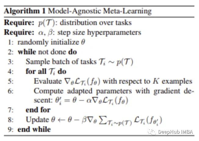
Model-Agnostic Meta-Learning (MAML)

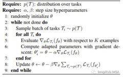
The gradient-based meta-learning (GBML) principle underpins MAML. In GBML, the meta-learner gains prior experience by training the base model and learning the shared features of all task representations. Whenever there is a new task to learn, the meta-learner fine-tunes training using its existing experience and the minimal new training data provided by the new task.

Generally, if we randomly initialize parameters, the algorithm will not converge to good performance after several updates. MAML attempts to solve this problem. MAML provides a reliable initialization for the meta-parameter learner with just a few gradient steps and guarantees no overfitting, enabling optimal rapid learning for new tasks.

The steps are as follows:

The meta-learner creates its copy C at the start of each episode,

C is trained on this episode (with the help of the base model),

C predicts on the query set,

The loss calculated from these predictions is used to update C,

This process continues until all episodes are trained.

1. The meta-learner creates its copy C at the start of each episode,

2. C is trained on this episode (with the help of the base model),

3. C predicts on the query set,

4. The loss calculated from these predictions is used to update C,

5. This process continues until all episodes are trained.

The main advantage of this technique is that it is considered independent of the choice of meta-learning algorithms. Therefore, the MAML method is widely used in many machine learning algorithms that require rapid adaptation, especially deep neural networks.

Matching Networks

The first metric learning method created to solve the FSL problem is Matching Networks (MN).

When using the matching network method to solve the Few-Shot Learning problem, a large base dataset is required. After dividing this dataset into several episodes, for each episode, the matching network performs the following operations:

• Each image from the support set and query set is fed into a CNN, which outputs feature embeddings for them.

• The query images use the model trained on the support set to obtain the cosine distances of the embedded features, classified through softmax.

• The cross-entropy loss of the classification results is backpropagated to update the feature embedding model through the CNN.

In this way, matching networks can learn to construct image embeddings. MN can classify photos using this method without any special class prior knowledge. It simply compares a few instances of classes.

Since classes vary by episode, matching networks compute image attributes (features) that are crucial for class distinction. In contrast, standard classification algorithms select features unique to each class.

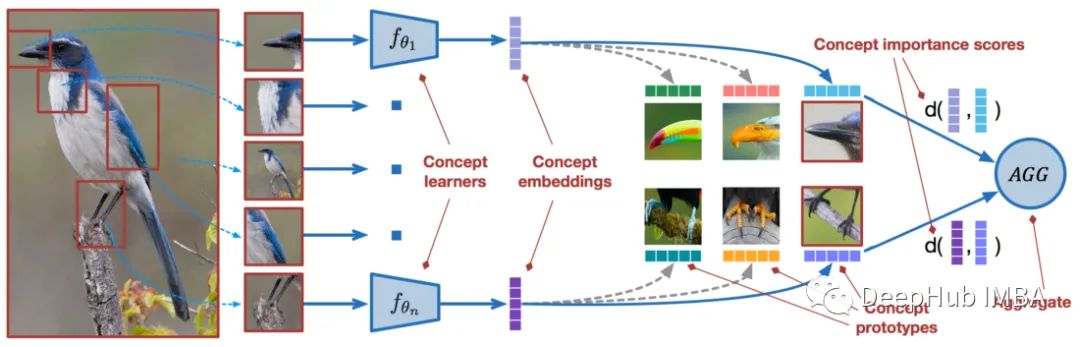
Prototypical Networks

Similar to matching networks are Prototypical Networks (PN). It improves the algorithm’s performance through some subtle changes. PN achieves better results than MN, but their training processes are essentially the same, merely comparing some query image embeddings from the support set; however, Prototypical Networks provide a different strategy.

In PN, we need to create class prototypes: class embeddings created by averaging the embeddings of images in the class. These class prototypes are then used to compare with the query image embeddings. When used for one-shot learning problems, it can rival matching networks.

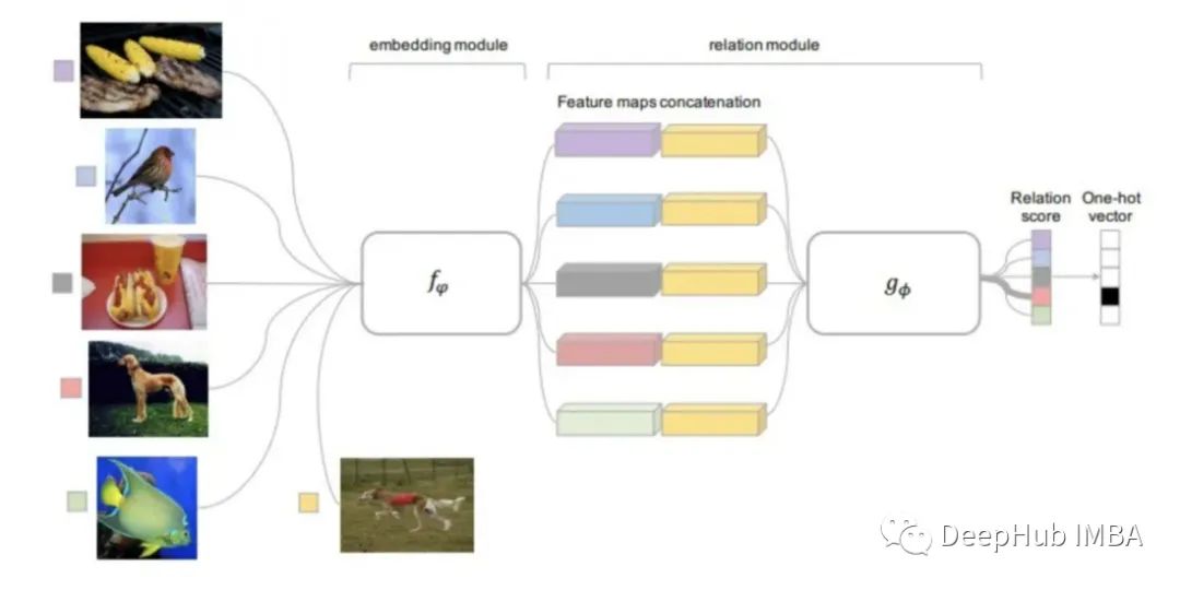
Relation Networks

Relation Networks can be said to inherit the results of the research from all the methods mentioned above. RN is based on the PN idea but includes significant algorithmic improvements.

The distance function used in this method is learnable, rather than being predefined as in previous studies. The relation module is located above the embedding module, which computes the embeddings and class prototypes from the input images.

The trainable relation module (distance function) takes as input the embeddings of the query images and each class prototype, outputting a relation score for each classification match. The relation score is obtained through Softmax to yield a prediction.

Zero-Shot Learning Using Open-AI CLIP

CLIP (Contrastive Language-Image Pre-Training) is a neural network trained on various (image, text) pairs. It can predict the most relevant text segments for a given image without being directly optimized for the task, similar to the zero-shot capabilities of GPT-2 and 3.

CLIP can achieve the performance of the original ResNet50 on ImageNet “zero-shot” without using any labeled examples, overcoming several major challenges in computer vision. Below we use PyTorch to implement a simple classification model.

Importing Packages

! pip install ftfy regex tqdm
! pip install git+https://github.com/openai/CLIP.git
import numpy as np
import torch
from pkg_resources import packaging

print("Torch version:", torch.__version__)

Loading the Model

import clip
clip.available_models()  # it will list the names of available CLIP models
model, preprocess = clip.load("ViT-B/32")  
model.cuda().eval()  
input_resolution = model.visual.input_resolution  
context_length = model.context_length  
vocab_size = model.vocab_size  

print("Model parameters:", f"{np.sum([int(np.prod(p.shape)) for p in model.parameters()]):,}")  
print("Input resolution:", input_resolution)  
print("Context length:", context_length)  
print("Vocab size:", vocab_size)

Image Preprocessing

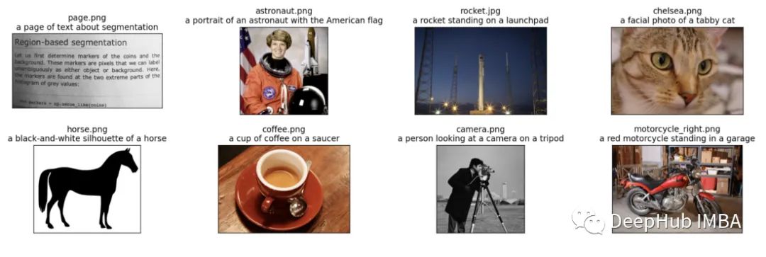
We will input 8 example images and their text descriptions to the model and compare the similarity between corresponding features.

The tokenizer is case-insensitive, allowing us to provide any suitable text description.

import os  
import skimage  
import IPython.display  
import matplotlib.pyplot as plt  
from PIL import Image  
import numpy as np  

from collections import OrderedDict  
import torch  

%matplotlib inline  
%config InlineBackend.figure_format = 'retina'  

# images in skimage to use and their textual descriptions  
descriptions = {  
   "page": "a page of text about segmentation",  
   "chelsea": "a facial photo of a tabby cat",  
   "astronaut": "a portrait of an astronaut with the American flag",  
   "rocket": "a rocket standing on a launchpad",  
   "motorcycle_right": "a red motorcycle standing in a garage",  
   "camera": "a person looking at a camera on a tripod",  
   "horse": "a black-and-white silhouette of a horse",  
   "coffee": "a cup of coffee on a saucer"  
}
original_images = []  
images = []  
txts = []  
plt.figure(figsize=(16, 5))  

for filename in [filename for filename in os.listdir(skimage.data_dir) if filename.endswith(".png") or filename.endswith(".jpg")]:  
    name = os.path.splitext(filename)[0]  
    if name not in descriptions:  
        continue  

    image = Image.open(os.path.join(skimage.data_dir, filename)).convert("RGB")  
       
    plt.subplot(2, 4, len(images) + 1)  
    plt.imshow(image)  
    plt.title(f"{filename}\n{descriptions[name]}")  
    plt.xticks([])  
    plt.yticks([])  
       
    original_images.append(image)  
    images.append(preprocess(image))  
    texts.append(descriptions[name])  

plt.tight_layout()  

Results Visualization:

We normalize the images, tokenize each text input, and run the model’s forward propagation to obtain the features of the images and texts.

image_input = torch.tensor(np.stack(images)).cuda()  
text_tokens = clip.tokenize(["This is " + desc for desc in texts]).cuda()  

with torch.no_grad():  
    image_features = model.encode_image(image_input).float()  
    text_features = model.encode_text(text_tokens).float()

We normalize the features and compute the dot product for each pair to perform cosine similarity calculations.

image_features /= image_features.norm(dim=-1, keepdim=True)  
text_features /= text_features.norm(dim=-1, keepdim=True)  
similarity = text_features.cpu().numpy() @ image_features.cpu().numpy().T  

count = len(descriptions)  

plt.figure(figsize=(20, 14))  
plt.imshow(similarity, vmin=0.1, vmax=0.3)  
# plt.colorbar()  
plt.yticks(range(count), texts, fontsize=18)  
plt.xticks([])  
for i, image in enumerate(original_images):  
    plt.imshow(image, extent=(i - 0.5, i + 0.5, -1.6, -0.6), origin="lower")  
for x in range(similarity.shape[1]):  
    for y in range(similarity.shape[0]):  
        plt.text(x, y, f"{similarity[y, x]:.2f}", ha="center", va="center", size=12)  

for side in ["left", "top", "right", "bottom"]:  
 plt.gca().spines[side].set_visible(False)  

plt.xlim([-0.5, count - 0.5])  
plt.ylim([count + 0.5, -2])  

plt.title("Cosine similarity between text and image features", size=20)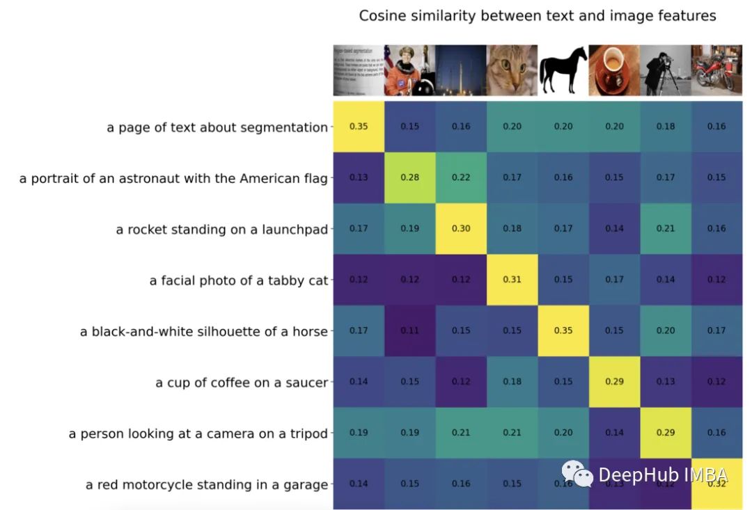

Zero-Shot Image Classification

from torchvision.datasets import CIFAR100  
cifar100 = CIFAR100(os.path.expanduser("~/.cache"), transform=preprocess, download=True)  
text_descriptions = [f"This is a photo of a {label}" for label in cifar100.classes]  
text_tokens = clip.tokenize(text_descriptions).cuda()  
with torch.no_grad():  
    text_features = model.encode_text(text_tokens).float()  
    text_features /= text_features.norm(dim=-1, keepdim=True)  

text_probs = (100.0 * image_features @ text_features.T).softmax(dim=-1)  
top_probs, top_labels = text_probs.cpu().topk(5, dim=-1)  
plt.figure(figsize=(16, 16))  
for i, image in enumerate(original_images):  
    plt.subplot(4, 4, 2 * i + 1)  
    plt.imshow(image)  
    plt.axis("off")  

    plt.subplot(4, 4, 2 * i + 2)  
    y = np.arange(top_probs.shape[-1])  
    plt.grid()  
    plt.barh(y, top_probs[i])  
    plt.gca().invert_yaxis()  
    plt.gca().set_axisbelow(True)  
    plt.yticks(y, [cifar100.classes[index] for index in top_labels[i].numpy()])  
    plt.xlabel("probability")  

plt.subplots_adjust(wspace=0.5)  
plt.show()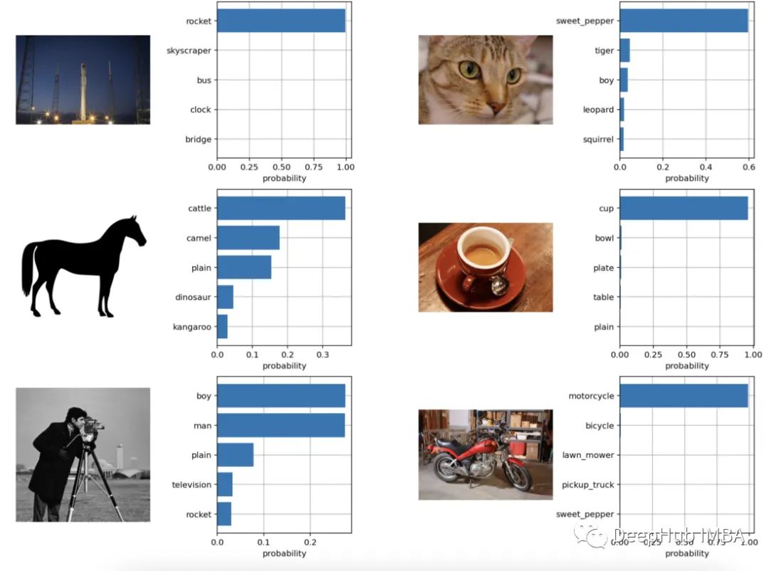

As we can see, the classification results are still very good.

Download 1: OpenCV-Contrib Extension Module Chinese Tutorial
Reply: Extension Module Chinese Tutorial in the "Beginner Learning Vision" public account backend to download the first OpenCV extension module tutorial in Chinese, covering more than twenty chapters including extension module installation, SFM algorithms, stereo vision, object tracking, biological vision, super-resolution processing, etc.

Download 2: Python Vision Practical Projects 52 Lectures
Reply: Python Vision Practical Projects in the "Beginner Learning Vision" public account backend to download 31 visual practical projects including image segmentation, mask detection, lane line detection, vehicle counting, eyeliner addition, license plate recognition, character recognition, emotion detection, text content extraction, face recognition, etc., to assist in quickly learning computer vision.

Download 3: OpenCV Practical Projects 20 Lectures
Reply: OpenCV Practical Projects 20 Lectures in the "Beginner Learning Vision" public account backend to download 20 practical projects based on OpenCV to achieve advanced learning in OpenCV.

Group Chat

Welcome to join the public account reader group to communicate with peers. Currently, there are WeChat groups on SLAM, 3D vision, sensors, autonomous driving, computational photography, detection, segmentation, recognition, medical imaging, GAN, algorithm competitions, etc. (will be gradually subdivided in the future). Please scan the WeChat ID below to join the group, and note: "Nickname + School/Company + Research Direction", for example: "Zhang San + Shanghai Jiaotong University + Visual SLAM". Please note the format; otherwise, you will not be approved. After successful addition, you will be invited into the relevant WeChat group based on your research direction. Please do not send advertisements in the group; otherwise, you will be removed from the group. Thank you for your understanding.~