Dialogue analysis uses output from:Using proxies to bring NPCs to life with CrewAI
Analysis
-
• Simulation 1: A group of software engineers, computer scientists, and computer engineers -
• Conclusion -
• Support
Analysis Methods
-
• Extracted Features -
• Split global_conversations.txt -
• Sentiment, Topic, Vocabulary Diversity, Emotion -
• Self-Similarity -
• Notebook
Background
Previously, I discussed in my articles Injecting Life into NPCs Using Proxies and Injecting Life into NPCs with CrewAI why I am interested in simulating two-dimensional societies. Let’s analyze a brief dialogue conducted using a dialogue party simulator. Note that this is prior to the development of any NPCs interacting with the world.
Population of Software Engineers, Computer Scientists, and Computer Engineers
We added NPCs with backgrounds in relevant research fields. Their initial tasks should enable them to easily discuss with each other.
NPCs
Non-playable characters in the simulation
Carly Cummings — Computer Scientist, Initial Task: Apply Bitwise Operations
Katherine Jones — Computer Engineer, Initial Task: Create Half Adder
Ashley Brown — Electrical Engineer, Initial Task: Apply Boolean Logic
Conclusion
-
• The three NPCs consistently revolve around the topic, or more specifically, they rarely deviate from the initial topic. -
• In specific dialogues, the range of vocabulary used is impressively diverse; however, echoes of the discussion can be seen in the responses, which is evident when comparing similarity between texts. -
• Topic analysis reveals two dialogues. It is important to note that this may be because the two individuals did not interact. The combinations of bidirectional dialogues are: Carly<->Katherine, Carly<-Ashley
Support
Text
The dialogue text can be found at the beginning of this notebook
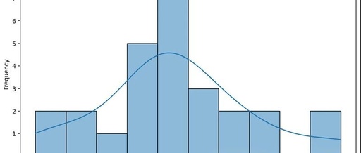
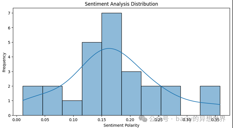
Sentiment Analysis:
Remember: -1 is negative, 0 is neutral, +1 is positive
From the analyzed dialogues, we can see that some very neutral and relatively positive dialogues occurred.
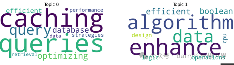
Topics
Identified two topic groups:
Topic 0 includes: ‘queries’, ‘caching’, ‘query’, ‘optimization’, ‘database’, ‘efficient’, ‘strategy’, ‘performance’, ‘retrieval’, ‘data’
Topic 1 includes: ‘enhancement’, ‘like’, ‘algorithm’, ‘data’, ‘efficient’, ‘boolean’, ‘operation’, ‘design’, ‘cpu’, ‘logic’
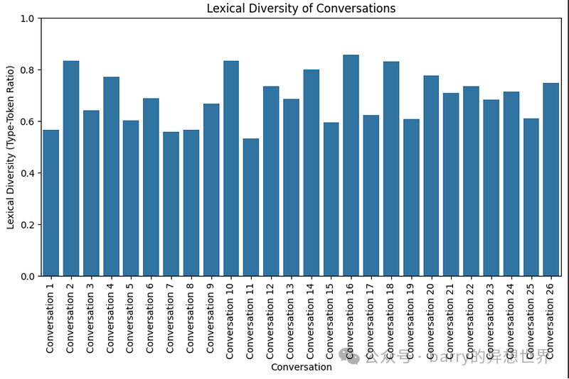
Vocabulary Diversity
Remember: This is the ratio of unique words to all words. In other words, as vocabulary diversity approaches 1 (maximum uniqueness), more words are unique; as vocabulary diversity approaches 0 (minimum uniqueness), more words are repeated.
We can see from this chart that the use of words in each dialogue has medium to high uniqueness.
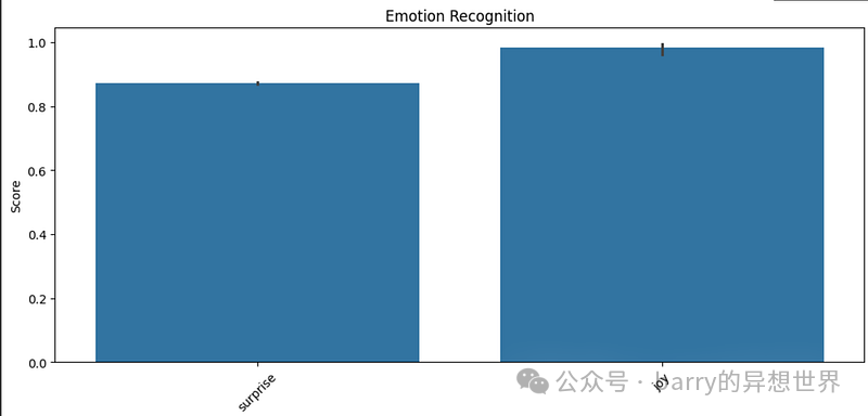
Emotion Recognition
Using Hugging Face Transformers for emotion recognition: emotion_pipeline = pipeline(‘sentiment-analysis’, model=’bhadresh-savani/distilbert-base-uncased-emotion’)
The identified emotions in the communication are surprise and joy.
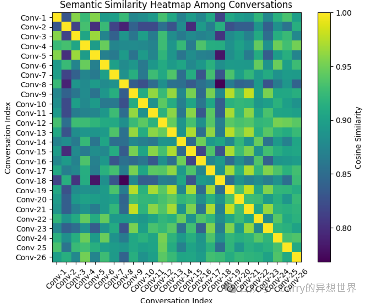
Semantic Similarity
Remember: 1 indicates complete similarity, while -1 indicates complete dissimilarity
Clearly, the conversations remain on similar topics; for example, our least similar cosine similarity is about 0.8, which is quite similar.
Analysis Methods
Extracted Features
-
1. Sentiment Analysis: Quick polarity assessment using TextBlob -
2. Topic Modeling: Using LDA to identify topics; ensure data preprocessing for better results (e.g., removing stop words, lemmatization). -
3. Vocabulary Diversity: Simple type-token ratio. -
4. Emotion Recognition: Using a BERT-based model on Hugging Face to identify emotions beyond simple sentiment. -
5. Semantic Similarity: Basic example of embedding similarity using BERT, indicating contextual alignment between dialogue turns.
Split global_conversations.txt
We have a pattern of who is talking to whom, so we split on these vectors; ignoring the speaker and audience
import re
def split_conversation(raw_conversation):

# Our dialogue is roughly "<person talking> (talking to <person>):..."
# Let's split based on this pattern
  lines = re.split(r'^.*?\(talking to.*?\):', raw_conversation, flags=re.MULTILINE)

# Remove empty lines and strip whitespace from each line
return [line.strip() for line in lines if line.strip()]
Emotion Themes and Sentiment
import nltk
nltk.download('punkt_tab')
nltk.download('punkt')
nltk.download('stopwords')
nltk.download('vader_lexicon')
import gensim
import numpy as np
import pandas as pd
from textblob import TextBlob
from sklearn.feature_extraction.text import CountVectorizer
from sklearn.decomposition import LatentDirichletAllocation
from nltk.corpus import stopwords
import transformers
from transformers import pipeline, BertTokenizer, BertModel
from gensim import corpora, models
from collections import Counter
import networkx as nx

def sentiment_analysis(conversations):
    sentiments = []
    for conversation in conversations:
        blob = TextBlob(conversation)
        sentiments.append(blob.sentiment.polarity)
    return sentiments

def topic_modeling(conversations, num_topics=2):
    cv = CountVectorizer(stop_words='english')
    dtm = cv.fit_transform(conversations)
    lda = LatentDirichletAllocation(n_components=num_topics, random_state=0)
    lda.fit(dtm)
    topic_results = lda.transform(dtm)
    topic_words = {}
    for i, topic in enumerate(lda.components_):
        topic_words[f"Topic {i}"] = [cv.get_feature_names_out()[j]
                                     for j in topic.argsort()[-10:]]
    return topic_words

def lexical_diversity(conversations):
    diversities = []
    for conversation in conversations:
        words = nltk.word_tokenize(conversation)
        diversity = len(set(words)) / len(words) #"set of words"/"num words"
        diversities.append(diversity)
    return diversities

### Use Hugging Face Transformers for emotion recognition
emotion_pipeline = pipeline('sentiment-analysis',
                            model='bhadresh-savani/distilbert-base-uncased-emotion')

def detect_emotions(conversation_texts):
    return emotion_pipeline(conversation_texts)

sentiments = sentiment_analysis(conversations)
topics = topic_modeling(conversations)
diversities = lexical_diversity(conversations)
emotions = detect_emotions(conversations)

print(f'Sentiments: {sentiments}')
print(f'Topics: {topics}')
print(f'Lexical Diversities: {diversities}')
print(f'Emotions: {emotions}')
Self-Similarity
We initialize a BERT tokenizer and model from Hugging Face transformers, which are pre-trained on the “bert-base-uncased” corpus to compute semantic similarity between a given list of texts. The get_embeddings() function tokenizes sentences, generates their embeddings using BERT, and averages the vectors to produce a single embedding. The calculate_cosine_similarity() function computes the cosine similarity between two embedding vectors, quantifying their semantic similarity. The semantic_similarity() function processes all dialogues, obtains their embeddings, and fills a matrix with pairwise cosine similarities. When filling the matrix, be sure to set self-similarity comparisons to 1.0. This matrix forms the basis of a heatmap, where yellow indicates more similarity and blue indicates less similarity.
from transformers import BertTokenizer, BertModel
import torch
import numpy as np
import matplotlib.pyplot as plt

### Init BERT tokenizer and model
tokenizer = BertTokenizer.from_pretrained('bert-base-uncased')
model = BertModel.from_pretrained('bert-base-uncased')

def get_embeddings(sentence):
    inputs = tokenizer(sentence, return_tensors='pt', truncation=True, padding=True)
    with torch.no_grad():
        outputs = model(**inputs)
    return outputs.last_hidden_state.mean(dim=1).squeeze()

def calculate_cosine_similarity(embed1, embed2):
    cos_sim = np.dot(embed1, embed2) / (np.linalg.norm(embed1) * np.linalg.norm(embed2))
    return cos_sim

def semantic_similarity(conversations):
    embeddings = [get_embeddings(conversation).numpy() for conversation in conversations]
    similarities = np.zeros((len(conversations), len(conversations)))

    for i in range(len(conversations)):
        for j in range(len(conversations)):
            if i != j:
                similarities[i][j] = calculate_cosine_similarity(embeddings[i], embeddings[j])
            else:
                similarities[i][j] = 1.0 # Similarity of a sentence with itself

    return similarities

### Calculate semantic similarities for the entire conversation set
similarities = semantic_similarity(conversations)

### Semantic similarity as a heatmap
plt.figure(figsize=(8, 6))
plt.imshow(similarities, cmap='viridis', interpolation='nearest')
plt.colorbar(label='Cosine Similarity')
plt.xticks(ticks=range(len(conversations)), labels=[f"Conv-{i+1}" for i in range(len(conversations))], rotation=45)
plt.yticks(ticks=range(len(conversations)), labels=[f"Conv-{i+1}" for i in range(len(conversations))])
plt.title('Semantic Similarity Heatmap Among Conversations')
plt.xlabel('Conversation Index')
plt.ylabel('Conversation Index')
plt.show()
Notes
If you find this article enlightening, please consider liking it — this not only supports the author but also helps others discover valuable insights. Also, don’t forget to subscribe for more in-depth articles on innovative technologies and developments in artificial intelligence. Thank you very much for your participation!