
Selected from blog.bradfieldcs
Author:Tyler Elliot Bettilyon
Translated by Machine Heart
Hash algorithms have always been one of the most classic methods for indexing, allowing for efficient storage and retrieval of data. However, in December of last year, Jeff Dean and researchers from MIT viewed indexing as a model, exploring conditions under which deep learning models outperform traditional indexing structures. This article will first introduce what indexing and hash algorithms are, and describe how viewing indexing as a model learning can be a more efficient representation than hash algorithms in the era of machine learning and deep learning.
In December 2017, researchers from Google and MIT published a research paper titled “The Case for Learned Index Structures,” which discusses their explorations in the field of “learned index structures.” This research is very exciting, as the authors noted in the abstract:
“[…] We believe that the idea of replacing core components of data management systems with learnable models has far-reaching implications for the design of future systems, and our work is merely a glimpse of what is to come.”
Indeed, the research proposed by Google and MIT can rival the most classic and effective structures in the indexing world, such as B-Trees and Hash Maps. The engineering community has long had many views on the future of machine learning, and thus, this research paper has gained widespread attention and discussion on Hacker News, Reddit, and all industrial forums around the world.
The new research presents an excellent opportunity to re-examine the fundamentals of a field, and foundational technologies like indexing, which have already been sufficiently studied, rarely have the chance for significant breakthroughs. This article serves as an introductory overview of hash tables, briefly introducing the main factors affecting their speed, and providing an intuitive understanding of machine learning concepts applied to indexing construction techniques.
In response to the work published by Google/MIT, Peter Bailis and a research team from Stanford reviewed the basics of index construction and urged us not to discard classic algorithm books. Bailis and his team at Stanford reconstructed learned index strategies and achieved similar results without using any machine learning techniques by employing a classic hash table strategy known as Cuckoo Hashing.
In another response to the work published by Google/MIT, Thomas Neumann described another way to achieve performance similar to learned index strategies, which still utilized the well-tested and deeply understood B-Tree. Of course, these discussions, comparative experiments, and calls for further research are precisely why the Google/MIT team is excited; they wrote in their paper:
“It is important to emphasize that we are not calling for a complete replacement of traditional indexing structures with learned index structures. Rather, we have outlined a new method for index construction that can fill the gaps in existing work, and can even be said to open a new research direction in a field that has been studied for decades.”
So, what has sparked such interest? Are hash maps and B-Trees destined to be replaced by new technologies? Are machines about to rewrite the algorithm textbooks? If machine learning strategies are indeed better than the general indexing strategies we know and love, what does that mean for the computing world? Under what conditions will learned indexing surpass old indexing methods?
To address these questions, we need to understand what indexing is, what problems they solve, and what determines the differences in advantages and disadvantages between different indices.
What is Indexing
The core of indexing is to enhance the convenience of information querying and retrieval. Long before the invention of computers, humans have been indexing things. When we use neat filing cabinets, we are using an indexing system. A complete encyclopedia can be seen as a form of indexing strategy, and the labeled aisles in a grocery store are also a form of indexing. When we have many items and need to find or identify a specific item within a collection, indexing can make the querying process more efficient and convenient.
Zenodotus, the first librarian of the Library of Alexandria, was responsible for organizing and managing the library’s vast collection. The system he designed included grouping books by genre into rooms and arranging them alphabetically. His contemporary Callimachus went further by introducing a central catalog called pinakes, which allowed librarians to look up authors and determine the location of each of that author’s books in the library. Many indexing methods have been invented, including the Dewey Decimal System, which was invented in 1876.
In the Library of Alexandria, indexing was used to map a piece of information (the name of a book or author) to a physical location within the library. Although our computers are digital devices, any specific data in a computer actually resides at least in one physical location. Whether it is text, recent credit card transaction records, or videos, data exists at a specific physical disk location on the computer.
In RAM and solid-state drives, data is stored as voltage in a series of transistors. In older rotating hard drives, data is stored in a specific arc on the disk in disk format. When we index information in a computer, we create some algorithms that map portions of data to physical locations in the computer. We refer to this address as the address. In a computer, all indexed information exists as data in the form of bits, and indexing is used to map this data to their addresses.
Databases are a typical use case for indexing. Databases are designed to store large amounts of information, and generally, we want to retrieve this information efficiently. The core of search engines is a vast index of the information available on the internet, and hash tables, binary search trees, trie trees, B-trees, and bloom filters are all forms of indexing.
It is easy to imagine how difficult it would be to find a specific book in the maze-like halls of the Library of Alexandria, but we should not take for granted that the size of data generated by humans is growing exponentially. The amount of data available to people on the internet far exceeds the capacity of any single library at any time, and Google’s goal is to index all data. Humans have created many strategies for indexing, and in this article, we discuss one of the most productive data structures in history, which happens to be a form of indexing structure: the hash table.
What is a Hash Table
At first glance, a hash table is a simple data structure based on hash functions, and there are many different hash functions used for various purposes. In the following sections, we will only describe the hash functions used in hash tables and will not discuss cryptographic hash functions, checksums, or any other types of hash functions.
A hash function takes some input values (such as numbers or text) and returns an integer, which we refer to as a hash code or hash value. For any given identical input, the hash code is always the same, meaning that the hash function must be deterministic.
When constructing a hash table, we first allocate some space for the hash table (in memory or on disk), which we can think of as creating a new array of arbitrary size. If we have a lot of data, we may use a larger array; if we have only a small amount of data, we can use a smaller array. Whenever we want to index a single piece of data, we need to create a key-value pair, where the key is some identifying information about the data, and the value is the data itself.
We need to insert the value into the hash table by sending the key of the data to the hash function. The hash function returns an integer (hash code), and we use this integer (modulo the size of the array) as the storage index for the value in our array. If we want to retrieve a value from the hash table, we simply recalculate the hash code from the key and retrieve the data from that position in the array, which is the physical address of our data.
In a library using the Dewey Decimal System, the “key” is the series of classifications that the book belongs to, and the “value” is the book itself. The “hash code” is the numerical value created through the Dewey Decimal process, for example, a book on analytic geometry has a hash code of 516.3, where natural sciences are 500, mathematics is 510, geometry is 516, and analytic geometry is 516.3. In this way, the Dewey Decimal System can be seen as a hash function for books, and these books will be placed on the shelves corresponding to their hash values, sorted alphabetically by the author within the shelves.
Our analogy is not particularly perfect; unlike Dewey Decimal numbers, the hash values used for indexing in a hash table typically do not convey information—ideally, the library catalog would contain the exact location of each book based on some relevant information (perhaps its title, the author’s surname, or its ISBN…), but unless all books with the same key are placed on the same shelf and we can use the key to find the shelf number in the library catalog, the grouping or sorting of books is meaningless.
Fundamentally, this simple process is all accomplished by the hash table. However, to ensure the correctness and efficiency of the hash index, we have built many complex components on top of this.
Performance Considerations for Hash-Based Indexing
The main source of complexity and optimization in hash tables is the issue of hash collisions. A collision occurs when two or more keys produce the same hash code. Consider the following simple hash function, assuming the keys are integers:
function hashFunction(key) {
  return (key * 13) % sizeOfArray;
}
While any unique integer will produce a unique result when multiplied by 13, due to the pigeonhole principle, we cannot place 6 items into 5 buckets without putting at least one item in the same bucket. Because our storage capacity is limited, we have to use the hash value modulo the size of the array, which means we will always encounter collisions.
We will soon discuss common strategies for handling these inevitable collisions, but it should first be noted that the choice of hash function can increase or decrease the likelihood of collisions. Imagine we have a total of 16 storage locations and must choose one of the following two functions as a hash function:
function hash_a(key) {
  return (13 * key) % 16;
}

function hash_b(key){
  return (4 * key) % 16;
}
In this case, if we hash the numbers 0-32, hash_b will produce 28 collisions or overlaps. Seven collisions occur at hash values 0, 4, 8, and 12 (the first four insertions do not collide, but every subsequent insertion will). However, hash_a will distribute collisions evenly, with each index colliding once, totaling 16 collisions. This is because in hash_b, 4 is a factor of the hash table size 16, while in hash_a, we chose a prime number, meaning unless our table size is a multiple of 13, we will not encounter the grouping problem seen with hash_b.
We can run the following script to observe this process:
function hash_a(key) {
  return (13 * key) % 16;
}

function hash_b(key){
  return (4 * key) % 16;
}

let table_a = Array(16).fill(0);
let table_b = Array(16).fill(0);

for(let i = 0; i < 32; i++) {
  let hash_code_a = hash_a(i);
  let hash_code_b = hash_b(i);

  table_a[hash_code_a] += 1;
  table_b[hash_code_b] += 1;
}

console.log(table_a); // [2,2,2,2,2,2,2,2,2,2,2,2,2,2,2,2]
console.log(table_b); // [8,0,0,0,8,0,0,0,8,0,0,0,8,0,0,0]
A good hash function can distribute hash code collisions more evenly across the table.
This hashing strategy, multiplying the input key by a prime number, is a very common practice. Primes reduce the likelihood that the output hash code shares a common factor with the size of the array, thereby reducing the chances of collisions. Since hash tables have been around for quite some time, there are many different excellent hash functions to choose from.
Multiplicative shift hashing is similar to the prime modulus strategy but avoids the relatively expensive modulus operation, favoring quick shift operations. MurmurHash and Tabulation Hashing are powerful alternatives in the multiplicative shift hashing family. Benchmarks for these hash functions include checking their computational speed, the distribution of generated hash codes, and their flexibility in handling different types of data (such as strings and floating-point numbers beyond integers).
If we choose a good hash function, we can lower the collision rate while maintaining high computational speed. Unfortunately, regardless of the hash function we choose, collisions are always unavoidable, and deciding how to handle collisions will significantly impact the overall performance of our hash table. Two common strategies for collision handling are chaining and linear probing.
Chaining is simple and easy to use; instead of storing each entry at every index in the hash table, we store a pointer to the head of a linked list. When an entry collides with an already filled index through our hash function, we add it as the last element in the linked list. Lookups are no longer strictly “constant time” since we must traverse the list to find a specific item. If our hash function has many collisions, we will have long chains. Additionally, due to the search for long chains, the performance of the hash table can degrade over time.
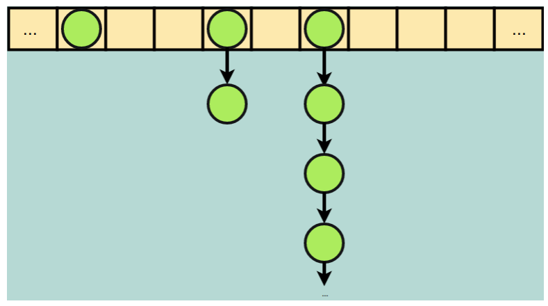
Chaining: repeated collisions create longer linked lists but do not occupy other indices in the array.
Linear probing is conceptually simple but can be tricky to implement. In linear probing, we still retain an index for each element in the hash table. When index i collides, we check if index i + 1 is empty; if so, we store the data there. If i + 1 also has an element, we check i + 2, then i + 3, and so on, until we find an empty slot. As long as we find an empty slot, we insert that value. Similarly, we may not achieve constant time complexity for lookups, and if multiple collisions occur at one index, we may end up searching through a long sequence before finding the entry we are looking for. More importantly, each time a collision occurs, the likelihood of subsequent collisions increases. Unlike chaining, every incoming item will eventually occupy a new index.

Linear probing: given the same data and hash function as above, we achieve a new result. Elements causing collisions (in red) now reside in the same array and occupy indices sequentially from the collision index.
It may sound like chaining is the better choice, but linear probing is often considered to have better performance characteristics. This is mostly due to the poor cache utilization of linked lists and the advantage of using arrays to improve cache utilization. In simple terms, checking all links in a linked list is much slower than checking all indices in an array of the same size. This is because indices in each array are physically adjacent, while each new node in a linked list is assigned a position when created. This new node is not necessarily physically adjacent to the previous node in the list. As a result, nodes that are “adjacent to each other” in the order of the list are not physically adjacent in RAM chips. Due to how CPU caches work, accessing adjacent memory locations is very fast, while accessing random memory locations is much slower.
Basics of Machine Learning
To understand how machine learning reconstructs the key features of hash tables (and other indices), it is necessary to quickly revisit the main ideas of statistical models. In statistics, a model is a function that accepts some vectors as input and returns labels (classification models) or data values (regression models). The input vectors contain relevant information about all data points, and the output labels or data are the predicted values of the model.
In a model predicting whether college students can enter Harvard, the input vector might include the student’s GPA, SAT scores, the number of extracurricular clubs they participate in, and other values related to academic achievement; the output label could be True or False (can enter Harvard or cannot enter Harvard).
In a model predicting mortgage default rates, the input vector might include credit scores, the number of credit card accounts, frequency of late payments, annual income, and other values related to the applicant’s financial situation, and the model would return a number within a range of 0 to 1 representing the likelihood of default.
In general, statistical models can be built using machine learning. Machine learning practitioners combine large datasets with machine learning algorithms, running the algorithms on the datasets to produce trained models. The core of machine learning lies in creating algorithms that can automatically build accurate models from raw data without human assistance to help the machine “understand” what the data actually represents. This is different from other forms of artificial intelligence, where humans extensively examine data, tell the computer what the data means (such as defining heuristics), and define how the computer should use that data (such as using minimax algorithms or A* pathfinding algorithms). Although in practice, machine learning is often combined with classic non-learning techniques; AI agents generally use both learning and non-learning strategies to achieve their goals.
Take the famous AI chess player “Deep Blue” and the recently popular AI Go player “AlphaGo” as examples. Deep Blue is a completely non-learning AI; programmers and chess experts collaborated to create a function for Deep Blue that takes the state of the chessboard as input (the positions of all pieces and the turn of the player) and returns a value related to how “good” that position is. Deep Blue never “learns” anything—human chess players wrote the machine’s evaluation function. The main feature of Deep Blue is its tree search algorithm, which calculates all possible moves and the possible responses from the opponent to those moves, as well as future possible moves.
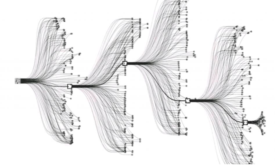
Visualization of AlphaGo’s tree search. (Source: https://blogs.loc.gov/maps/category/game-theory/)
AlphaGo also performs tree search. Similar to Deep Blue, AlphaGo predicts several moves ahead after considering possible moves, but differs in that AlphaGo establishes its own evaluation function without explicit guidance from Go experts. In this case, the evaluation function is a trained model. AlphaGo’s machine learning algorithm takes the state of the board (each position is either black, white, or empty) as the input vector, with labels indicating which player’s (white or black) move will win. Using this information, the machine learning algorithm can determine how to evaluate the current state based on millions of examples learned from playing many games.
Indexing as a Model, Deviating from the ML Paradigm
Google’s researchers first proposed in their paper that indexing is a model premise, or at least that machine learning models can be treated as indices. The reasoning is that models accept some input and return a label; if the input is a keyword and the label is the model’s judgment of the memory address, the model can act as an index. Although this sounds clear and straightforward, the issue of indexing seems not to fit perfectly with machine learning. In some fields, the Google team has deviated from the machine learning paradigm to achieve their goals.
In general, machine learning models are trained on known data with the goal of evaluating unseen data. If we index data, we cannot accept evaluation values. The only use of indexing is to obtain the precise location of some data in memory. A neural network (or other machine learning model) outside a box cannot be precise to that extent. Google addresses this issue by tracking maximum (positive) and minimum (negative) errors during training. Using these values as boundaries, ML indexing can search within the bounds to find the exact position of elements.
Another departure point is that machine learning practitioners generally need to be careful to avoid their models from “overfitting” the training data; an “overfitted” model may produce very high prediction accuracy on the training data but perform poorly on data outside the training set. On the other hand, indexing is by definition overfitting. The training set is the data that has been indexed, which also makes it the test set. Since lookups must occur on the actual data indexed, it is easier to encounter overfitting issues in this application of machine learning. Additionally, if the model has already overfitted the existing data, adding items to the index may cause terrible errors during prediction; as stated in the article:
“An interesting trade-off occurs between the universality of this model and its performance on the ‘last mile’; it can be said that the better the prediction results for the ‘last mile’, the more severe the model’s overfitting becomes, making it less applicable to new data items.”
Finally, in general, the training process of a model is the most expensive part of the entire process. Unfortunately, in widespread database applications (and other indexing applications), it is common to add data to the index. The team admits to this limitation:
“So far, our results have focused on index structures for read-only storage database systems. As we have pointed out, the current design, even without major modifications, can already replace the index structures in current databases—the former’s index structure may only be updated once a day, while the latter needs to create B-trees in bulk during the merging of SSTables.”—(SSTable is an important component of Google’s BigTable)
Learning Hashing
This article explores the possibility of using machine learning models to replace standard hash functions. One of the questions researchers want to understand is: can understanding the distribution of data help us better create indices? Traditional strategies (multiplicative shift, Murmur Hash, prime multiplication…) completely ignore the distribution of data. Each incoming item is treated as an independent value rather than considered as part of a larger dataset with numerical attributes. The result is that even in many advanced hash tables, there is a significant issue of wasted space.
The memory utilization of hash tables is only about 50%, meaning that the hash table occupies twice the actual space needed for data storage. In other words, when we store as many items as are stored in the array, half of the addresses are empty. By replacing the hash function in standard hash tables with a machine learning model, researchers found that wasted space was significantly reduced.
This is not particularly surprising: by training on the input data, the learned hash function can distribute values more evenly in some space because the ML model already knows the distribution of the data! This is a powerful way to significantly reduce the storage required for hash-based indexing. There are also some limitations: ML models are slower to compute than the standard hash functions described above and require training, while standard hash functions do not.
Perhaps ML-based hash functions can be used in situations where effective memory usage is critical, but in these situations, computational power is no longer a bottleneck. The Google and MIT research teams believe that databases are a good example because indices are rebuilt daily in a costly process; using more computational time to achieve significant memory savings is a win for many database environments.
But here, we still need a super expansion, moving on to Cuckoo Hashing.
Cuckoo Hashing
Cuckoo Hashing was invented in 2001 and is named after the cuckoo bird. Cuckoo Hashing is an alternative to handling hash collisions using chaining techniques and linear probing (rather than a replacement for hash functions). The strategy is aptly named because in some cuckoo species, the female preparing to lay eggs finds a nest with an owner, removes the eggs in that nest, and lays her own eggs inside. In Cuckoo Hashing, incoming data will steal the address of old data, just as cuckoos steal the nests of other birds.
The way it works is as follows: when creating a hash table, the table is divided into two spaces, referred to as the primary address space and the secondary address space. Then, two hash functions are initialized, with each function assigned to one address space. These hash functions may be very similar—for example, they may both belong to “prime multiplication,” with each hash function using a different prime. Let’s call these two functions the primary hash function and the secondary hash function.
Initially, inserting into Cuckoo Hashing will only utilize the primary hash function and the primary address space. When a hash collision occurs, the new data will evict the old data, which will then be hashed using the secondary hash function and placed in the secondary address space.
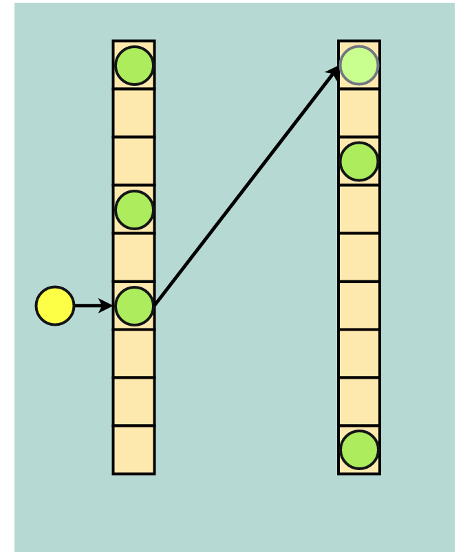
Cuckoo Hashing for handling hash collisions: yellow data evicts green data, and green data finds a new home in the secondary address space (the light green dot at the top of the secondary space index).
If that secondary address is already occupied, another eviction will occur, and the data in the secondary space will be sent back to the primary address space. Because there is a possibility of infinite eviction loops, a threshold for eviction attempts is generally set; if the number of evictions reaches the threshold, the hash table will be rebuilt, which may involve allocating more space for the table or choosing new hash functions.
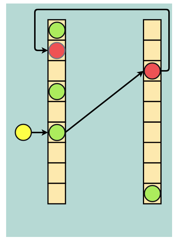
Double eviction: the incoming yellow dot evicts the green one, the green evicts the red one, and the red dot finds a home in the primary address space (light red dot).
This strategy is known to be very effective in memory-constrained situations. The so-called “power of two choices” allows Cuckoo Hashing to maintain stable performance even at high utilization rates (which is not the case with chaining techniques or linear probing).
Bails and his research team at Stanford found that with proper optimization, Cuckoo Hashing can be very fast, even achieving good performance with utilization rates as high as 99% (http://dawn.cs.stanford.edu/2018/01/11/index-baselines/). Essentially, Cuckoo Hashing achieves a high level of “machine learning” utilization without the expensive training phase by leveraging the power of two choices.
What is the Next Step for Indexing?
Ultimately, everyone is excited about the potential of learned index structures. With the broader application of more ML tools, as well as hardware advancements like TPUs that make machine learning workloads faster, indexing can greatly benefit from machine learning strategies. Meanwhile, elegant algorithms like Cuckoo Hashing remind us that machine learning is not a panacea. The work that combines incredibly powerful machine learning techniques with old theories like “the power of two” will continue to push the boundaries of computing efficiency and capability.
It seems that the fundamental principles of indexing will not be replaced overnight by machine learning strategies, but the idea of fine-tuning indexing is a powerful and exciting concept. As we become more adept at using machine learning and continually strive to improve the efficiency of computer processing of machine learning workloads, new ideas that leverage these advantages will surely find their mainstream applications. The next generation of DynamoDB or Cassandra may also leverage machine learning strategies well; applications of PostgreSQL or MySQL in the future may also adopt such strategies. Ultimately, it all depends on the achievements that future research can attain, which will continue to build on the cutting-edge non-linear strategies and the forefront technologies of the “AI revolution.”
For the sake of necessity, this article simplifies many details. Readers who wish to know more details can refer to:
-
The Case For Learned Indexes (Google/MIT) (https://www.arxiv-vanity.com/papers/1712.01208/)
-
Don’t Throw Out Your Algorithms Book Just Yet: Classical Data Structures That Can Outperform Learned Indexes (Stanford) (http://dawn.cs.stanford.edu/2018/01/11/index-baselines/)
-
A Seven-Dimensional Analysis of Hashing Methods and its Implications on Query Processing (https://bigdata.uni-saarland.de/publications/p249-richter.pdf) (Saarland University)
Original link: https://blog.bradfieldcs.com/an-introduction-to-hashing-in-the-era-of-machine-learning-6039394549b0
This article is translated by Machine Heart, Please contact this public account for authorization to reprint.
✄————————————————
Join Machine Heart (Full-time reporter/intern): [email protected]
Submissions or seeking coverage: [email protected]
Advertising & Business Cooperation: [email protected]