
Source: OneFlow


This article is approximately 3,611 words long and suggests a reading time of 7 minutes.
This article introduces the construction of AI large models and the four strategies of parallel computing.
Many recent advancements in the field of AI revolve around large-scale neural networks, but training these large-scale neural networks is a daunting engineering and research challenge that requires coordinating GPU clusters to perform a single synchronous computation.As the number of clusters and the scale of the model grow, machine learning practitioners have developed several techniques for parallel model training across multiple GPUs.At first glance, these parallel techniques may seem intimidating, but with some assumptions about the computational structure, they become clear—at this point, it’s just like packets being transmitted between network switches, which is merely a non-transparent transfer of bits from A to B.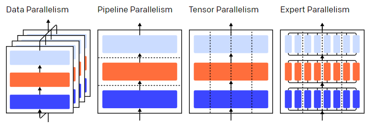
The parallel strategies in a three-layer model. Each color represents a layer, and the dashed lines separate different GPUs.
Training a neural network is an iterative process. During one iteration, the training data is fed forward through the model’s layers to compute the output for a batch of training samples. Then, it is passed backward through the layers, where the gradients of the parameters are computed to determine the influence of each parameter on the final output.
The batch average gradients, parameters, and the optimization state for each parameter are passed to the optimization algorithm, such as Adam, which calculates the parameters for the next iteration (for better performance) and updates the optimization state for each parameter. Through multiple iterations of training on the data, the training model continuously optimizes, yielding more precise outputs.
Different parallel techniques divide the training process into different dimensions, including:
- Data Parallelism— running different subsets of the same batch of data on different GPUs;
- Pipeline Parallelism— running different layers of the model on different GPUs;
- Tensor Parallelism— splitting a single mathematical operation (like matrix multiplication) across different GPUs;
- Mixture-of-Experts— using only a small portion of the model in each layer to process data.
This article takes GPU training of neural networks as an example, but the parallel techniques are also applicable to training with other neural network accelerators. The authors are Chinese engineer Lilian Weng and co-founder & president Greg Brockman from OpenAI.
1. Data Parallelism
Data parallelism refers to copying the same parameters to multiple GPUs, commonly referred to as “workers,” and assigning different subsets of data to each GPU for simultaneous processing. Data parallelism requires loading the model parameters into a single GPU’s memory, while the cost of computing across multiple GPUs means storing multiple copies of the parameters. That said, there are methods to increase the GPU’s RAM, such as temporarily offloading parameters to the CPU’s memory during unused intervals. When updating the parameter copies corresponding to the data parallel nodes, coordination is needed to ensure that each node has the same parameters. The simplest method introduces blocking communication between nodes: (1) compute gradients separately on each node; (2) compute the average gradients between nodes; (3) compute the same new parameters on each node separately. Among these, step (2) is a blocking average that requires transferring large amounts of data (proportional to the number of nodes multiplied by the size of the parameters), which can harm training throughput. Some asynchronous update schemes can eliminate this overhead, but they can compromise learning efficiency; in practice, synchronous update methods are usually employed.
2. Pipeline Parallelism
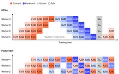
Pipeline parallelism refers to sequentially splitting the model into different parts to run on different GPUs. Each GPU only has a portion of the parameters, thus proportionally reducing the GPU memory consumption for each part of the model. It is straightforward to divide a large model into several continuous layers. However, there is a sequential dependency between the inputs and outputs of the layers, so when one GPU waits for the output from its predecessor as its input, a naive implementation can lead to a lot of idle time. This idle time is referred to as “bubbles,” during which the idle machine could continue processing. 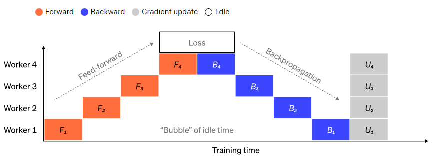 A naive pipeline parallel setup, where the model is vertically divided into 4 parts. Worker 1 hosts the model parameters of the first layer (closest to the input), while worker 4 hosts the parameters of the 4th layer (closest to the output). “F”, “B”, and “U” represent forward, backward, and update operations, respectively. The subscript indicates which node the data is running on. Due to sequential dependencies, data can only run on one node at a time, leading to significant idle time, or “bubbles.”To reduce the overhead of bubbles, the data parallel approach can be reused here, where the core idea is to split large batch data into several micro-batches, processing only one micro-batch at a time on each node, allowing new computations to occur during the original waiting times.Each micro-batch’s processing speed can be proportionally accelerated, allowing each node to start working as soon as the next micro-batch is released, thus speeding up the pipeline execution. With enough micro-batches, nodes are working most of the time, and bubbles are minimized at the beginning and end of the process. The gradients are the average of the micro-batch gradients, and parameters are updated only after all micro-batches are completed. The number of nodes for model splitting is usually referred to as pipeline depth. During the forward pass, nodes only need to send the output (activations) of their layer block to the next node; during the backward pass, nodes send these gradients of the activations back to the previous node. There is significant design space regarding how to schedule these processes and how to aggregate the gradients of the micro-batches. GPipe allows each node to continuously perform forward and backward passes while synchronizing and aggregating multiple micro-batch gradients at the end. PipeDream alternates between forward and backward passes on each node.
 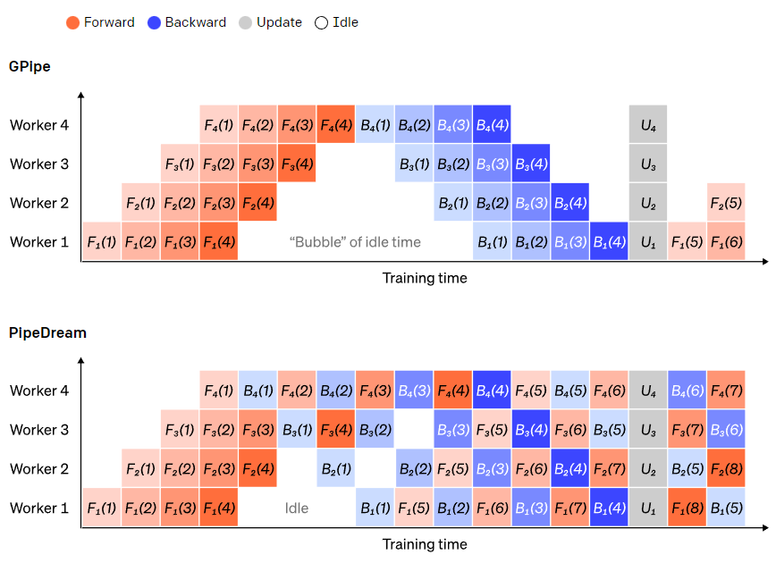 Comparison of GPipe and PipeDream pipeline schemes. Each batch of data is divided into 4 micro-batches, with micro-batches 1-8 corresponding to two consecutive large batches of data. In the figure, “(number)” indicates which micro-batch the operation is performed on, and the subscript denotes the node ID. Among them, PipeDream uses the same parameters for computations, achieving higher efficiency.
3. Model Parallelism
In pipeline parallelism, the model is “vertically” split along layers; if a single operation within a layer is “horizontally” split, this is model parallelism. Many modern models (like Transformer) have a computational bottleneck in multiplying activation values with weights.
Matrix multiplication can be viewed as several point products of rows and columns: independent point products can be computed on different GPUs, or parts of each point product can be computed on different GPUs and then summed to get the result.
Regardless of the strategy employed, the weight matrix can be divided into uniformly sized “shards,” with different GPUs responsible for different parts. To obtain the complete matrix result, communication is necessary to integrate the results from the different parts.
Megatron-LM performs parallel matrix multiplication on the self-attention and MLP layers of the Transformer; PTD-P simultaneously uses model, data, and pipeline parallelism, where pipeline parallelism allocates multiple non-contiguous layers to run on a single device at the cost of more network communication to reduce bubble overhead.
In certain scenarios, the network input can be parallelized across dimensions, allowing for higher degrees of parallel computation compared to cross-communication. For example, in sequence parallelism, the input sequence is divided temporally into multiple subsets, allowing for proportional reductions in peak memory consumption through finer-grained subset computations.
4. Mixture-of-Experts (MoE)
Mixture-of-Experts (MoE) models refer to using only a small portion of the network to compute the output for any given input. With multiple sets of weights, the network can choose which set of weights to use during inference through a gating mechanism, achieving more parameters without increasing computational costs.
Each set of weights is referred to as an “expert”; ideally, the network learns to assign specific computational tasks to each expert. Different experts can be hosted on different GPUs, providing a clear method for expanding the number of GPUs used for the model.
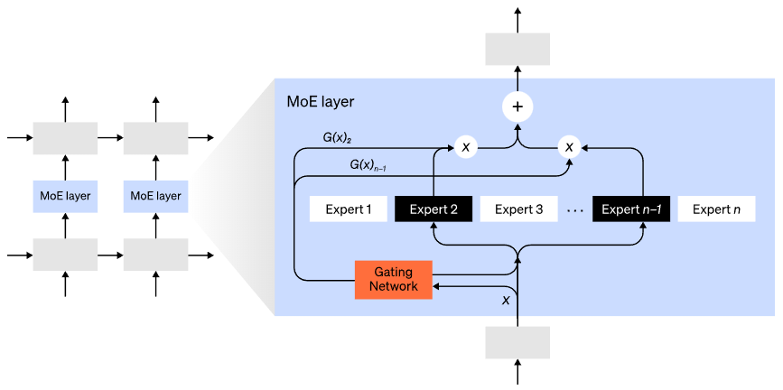
The Mixture-of-Experts (MoE) layer. The gating network selected only 2 out of n experts (image adapted from: Shazeer et al., 2017).
GShard expands the MoE Transformer to 600 billion parameters, where the MoE layers are split across multiple TPUs, while other layers are fully replicated. The Switch Transformer routes the input to only one expert, scaling the model size to trillions of parameters with higher sparsity.
5. Other Memory-Efficient Designs
In addition to the above parallel strategies, there are many other computational strategies that can be used to train large-scale neural networks:
- To compute gradients, the original activation values must be stored, which consumes a lot of device memory. Checkpointing (also known as activation recomputation) stores any subset of activations and recomputes intermediate activations during backpropagation as needed. This can save a significant amount of memory, with the computational cost being at most an additional complete forward pass. Selective activation recomputation can also be performed to continuously balance between computational and memory costs, checking those subsets of activations that have relatively high storage costs but low computational costs.
- Mixed Precision Training (https://arxiv.org/abs/1710.03740) uses lower precision numbers (typically FP16) to train models. Modern accelerators can achieve higher FLOP counts with low-precision numbers while also saving device memory. If handled properly, there is almost no loss in the accuracy of the generative model.
- Offloading involves temporarily unloading unused data to the CPU or other devices and reading it back when needed. A naive implementation can significantly reduce training speed, while a complex implementation can prefetch data, so the device does not have to wait for data. One implementation is ZeRO (https://arxiv.org/abs/1910.02054), which partitions parameters, gradients, and optimizer states across all available hardware and implements them as needed.
- Memory-Efficient Optimizers can reduce the memory of the running states maintained by the optimizer, such as Adafactor.
- Compression can be used to store intermediate results of the network. For example, Gist can compress activations saved for backpropagation; DALL·E can compress gradients before synchronizing them.
Original link:https://openai.com/blog/techniques-for-training-large-neural-networks/)——END——