Hinton's Latest Research: The Future of Neural Networks is Forward-Forward Algorithm

Big Data Digest authorized reprint from AI Technology Review

Authors: Li Mei, Huang Nan

Editor: Chen Caixian

In the past decade, deep learning has achieved remarkable victories, with methods using large parameters and data through stochastic gradient descent proven effective. The gradient descent typically uses the backpropagation algorithm, which has led to ongoing questions about whether the brain follows backpropagation and whether there are other ways to obtain the gradients needed to adjust connection weights.

Geoffrey Hinton, a Turing Award winner and pioneer of deep learning, one of the proposers of backpropagation, has repeatedly stated in recent years that backpropagation cannot explain how the brain works. Instead, he is proposing a new neural network learning method—the Forward-Forward Algorithm (FF).

At the recent NeurIPS 2022 conference, Hinton delivered an invited talk titled “The Forward-Forward Algorithm for Training Deep Neural Networks,” discussing the superiority of the forward algorithm compared to the backward algorithm. The preliminary draft of the paper “The Forward-Forward Algorithm: Some Preliminary Investigations” has been posted on his University of Toronto homepage:

Paper link:

https://www.cs.toronto.edu/~hinton/FFA13.pdf

Unlike the backpropagation algorithm, which uses one forward pass + one backward pass, the FF algorithm consists of two forward passes, one using positive (i.e., real) data and the other using negative data generated by the network itself.

Hinton believes that the advantage of the FF algorithm is that it can better explain cortical learning in the brain and can simulate hardware with extremely low power consumption.

Hinton advocates abandoning the separation of hardware and software in computer forms; future computers should be designed as “mortal,” significantly saving computing resources, and the FF algorithm is the best learning method that can run efficiently on such hardware.

This may be an ideal way to solve the computational bottleneck of trillion-parameter-level large models in the future.

FF Algorithm is More Energy Efficient and Explains the Brain Better than Backpropagation

In the FF algorithm, each layer has its own objective function, which has high goodness for positive data and low goodness for negative data. The sum of the squares of the activities in the layer can be used as goodness, and there are many other possibilities, such as subtracting the sum of the squares of the activities.

If positive and negative passes can be separated in a timely manner, then negative passes can be completed offline, making learning from positive passes simpler and allowing video to be transmitted through the network without storing activities or terminating propagation derivatives.

Hinton believes that the FF algorithm is superior to backpropagation in two aspects:

1. FF is a better model for explaining cortical learning in the brain;

2. FF is more energy-efficient, using extremely low power to simulate hardware without resorting to reinforcement learning.

There is no concrete evidence to prove that cortical propagation of erroneous derivatives or storing neural activities is used for subsequent backpropagation. The top-down connections from one cortical area to earlier areas in the visual pathway do not reflect the expected bottom-up connections when using backpropagation in the visual system. Instead, they form a cycle, where neural activity passes through two areas, about six cortices, and returns to where it started.

As one of the ways to learn sequences, the credibility of backpropagation through time is not high. To process sensory input streams without frequent pauses, the brain needs to transmit data through different stages that sensory processing entails, and it also needs a process that can learn in real-time. Later-stage representations in the pipeline may provide top-down information affecting early-stage representations, but the perceptual system needs to reason and learn in real-time, rather than stopping to perform backpropagation.

Among these, another serious limitation of backpropagation is that it requires a complete understanding of the calculations performed during forward propagation to derive correct derivatives. If we insert a black box into the forward propagation, backpropagation cannot execute unless we learn a differentiable model of the black box.

However, the black box does not affect the learning process of the FF algorithm because it does not require backpropagation through it.

When there is no perfect forward propagation model, we can start from various reinforcement learning methods. One idea is to introduce random perturbations to weights or neural activities and correlate these perturbations with changes in the resulting reward function. However, due to the high variance problem in reinforcement learning: when other variables are simultaneously perturbed, it is difficult to see the effect of perturbing a single variable. Therefore, to average out the noise caused by all other perturbations, the learning rate needs to be inversely proportional to the number of perturbed variables, which means that reinforcement learning has poor scalability and cannot compete with backpropagation, which contains millions or billions of parameters.

Hinton’s view is that neural networks with unknown non-linearities do not need to resort to reinforcement learning.

The FF algorithm can match the speed of backpropagation, and its advantage is that it can be used in cases where the precise details of forward computation are unknown, and it can learn while the neural network processes sequential data without storing neural activities or terminating propagation error derivatives.

However, in power-constrained applications, the FF algorithm has not yet replaced backpropagation, especially for extremely large models trained on ultra-large datasets, where backpropagation is still dominant.

Forward-Forward Algorithm

The Forward-Forward Algorithm is a greedy multi-layer learning program inspired by Boltzmann machines and noise-contrastive estimation.

Replacing backpropagation with two forward passes, the two forward passes operate on different data and opposing objectives in exactly the same way. The forward channel operates on real data and adjusts weights to increase the goodness of each hidden layer, while the backward channel adjusts the weights of “negative data” to reduce the goodness of each hidden layer.

This article explores two different metrics—the sum of squares of neural activities and the sum of squares of negative activities.

Assuming that the goodness function of a layer is the sum of squares of rectified linear neuron activities in that layer, the learning objective is to make its goodness far higher than a certain threshold for real data and far lower than a threshold for negative data. In other words, when the input vector is correctly classified as positive or negative data, the probability of the input vector being positive (i.e., real) can be obtained by applying the logistic function σ to the goodness minus a threshold θ:

Where,

is the activity of the hidden unit j before layer normalization. Negative data can be predicted by the neural network’s top-down connections or provided externally.

Layer-wise Optimization Function for Learning Multi-layer Representations

It is easy to see that a single hidden layer can be learned by having the sum of squares of the activities of hidden units high for positive data and low for negative data. However, when the activity of the first hidden layer is used as input to the second hidden layer, it is sufficient to use the length of the activity vector of the first hidden layer to distinguish positive and negative data without learning new features.

To prevent this, FF normalizes the hidden vector length before using it as input to the next layer, removing all information used to determine the first hidden layer, thereby forcing the next hidden layer to use the relative activity information of neurons in the first hidden layer, which is unaffected by layer normalization.

In other words, the activity vector of the first hidden layer has a length and a direction, where the length defines the goodness of that layer, and only the direction is passed to the next layer.

Experiments on FF Algorithm

Backpropagation Baseline

Most experiments in this paper used the MNIST dataset of handwritten digits: 50,000 for training, 10,000 for validation during the search for good hyperparameters, and 10,000 for calculating the test error rate. After designing a convolutional neural network with several hidden layers, a test error of about 0.6% can be achieved.

In the “translation invariant” version of the task, the neural network did not receive information about the pixel space layout, and if all training and testing images were affected by the same pixel random mutation before training began, the neural network’s performance would still be equally good.

For the “translation invariant” version of this task, the feedforward neural network with several fully connected hidden layers of rectified linear units (ReLU) had a test error of about 1.4%, requiring about 20 epochs to train. Using various regularizers such as dropout (which slows down training) or label smoothing (which speeds up training) can reduce the test error to around 1.1%. Furthermore, combining supervised learning of labels with unsupervised learning can further reduce the test error.

Without using complex regularizers, the test error for the “translation invariant” version of the task is 1.4%, indicating that its learning process is as effective as backpropagation.

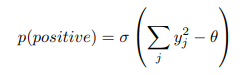
Figure 1: Mixed images used as negative data

Unsupervised FF Algorithm

FF has two main questions to answer: if there is a good source of negative data, can it learn effective multi-layer representations to capture the data structure? Where does the negative data come from?

First, use manual negative data to answer the first question. A common method for using contrastive learning in supervised tasks is to transform input vectors into representation vectors without using any label information, learning to transform these representation vectors into logits vectors used to determine the probability distribution of labels in softmax. Despite the obvious non-linearity, this is still referred to as a linear classifier, where the learning of the linear transformation of the logits vector is supervised, as it does not involve learning any hidden layers and does not require the derivatives of backpropagation. FF can perform this representation learning by using real data vectors as positive examples and corrupted data vectors as negative examples.

To make FF focus on the long-term correlations of shape images, we need to create negative data with different long-term correlations but very similar short-term correlations, which can be done by creating a mask containing a substantial area of 1s and 0s. Then, by adding a digit image to the mask, we create mixed images for negative data and multiply a different digit image by the inverse of the mask (Figure 1).

Starting with a random bitmap to create the mask, the image is repeatedly blurred using filters of the form [1/4, 1/2, 1/4] in both horizontal and vertical directions, and the threshold of the repeatedly blurred image is set to 0.5. After training for 100 epochs with four hidden layers (each containing 2000 ReLU), a test error of 1.37% can be achieved when using the normalized activity vector from the last three hidden layers as input for softmax.

Moreover, not using fully connected layers but using local receptive fields (without weight sharing) can improve performance, and after training for 60 epochs, a test error of 1.16% can be achieved. The architecture’s “peer normalization” prevents any hidden units from becoming overly active or permanently inactive.

Supervised Learning FF Algorithm

Learning hidden representations without using any label information is very wise for large models that may perform various tasks: unsupervised learning extracts a large number of features for various tasks. However, if only a single task is of interest and a small model is desired, supervised learning is more suitable.

One way to use FF in supervised learning is to include labels in the input, where positive data consists of images with the correct labels, and negative data consists of images with incorrect labels, with the labels being the only distinction between the two, and FF will ignore all features in the images that are unrelated to the labels.

MNIST images contain black borders that alleviate the workload of convolutional neural networks. When one of the N representations with labels replaces the first ten pixels, the content learned by the first hidden layer also becomes apparent. In a network with four hidden layers, each containing 2000 ReLU, fully connected between layers, after 60 epochs trained on MNIST, the test error is 1.36%, while backpropagation requires about 20 epochs to achieve this test performance. Doubling the FF learning rate and training for 40 epochs yields a slightly worse test error of 1.46%.

After training with FF, by starting with an input containing test digits and neutral labels composed of ten 0.1 entries, a forward pass through the network classifies the test digits, after which all hidden activities except the first hidden layer are used as softmax inputs learned during training, which is a fast suboptimal image classification method. The best way is to run the network with specific labels as part of the input, accumulating the advantages of all layers except the first hidden layer, and after performing this operation for each label, select the label with the highest accumulated goodness. During training, forward passes from the neutral labels are used to select hard negative labels, requiring about a third of the epochs for training.

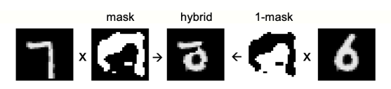
By using the two pixels that jitter the most in each direction to increase the training data, 25 different offsets are obtained for each image, utilizing knowledge of pixel space layout, making it no longer translation invariant. Training the same network on augmented data for 500 epochs yields a test error of 0.64%, similar to that of a convolutional neural network trained with backpropagation. In Figure 2, interesting local domains are also obtained in the first hidden layer.

Figure 2: Local domains of 100 neurons in the first hidden layer of the network trained on jittered MNIST images, with class labels shown in the first ten pixels of each image

Using FF to Simulate Top-down Perceptual Effects

Currently, all image classification cases use a feedforward neural network that learns one layer at a time, meaning that what is learned in later layers does not affect the learning of earlier layers. This seems to be a major weakness compared to backpropagation, and the key to overcoming this apparent limitation is to treat static images as relatively boring videos processed by multi-layer recurrent neural networks.

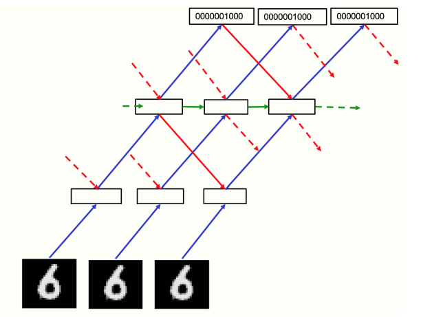
FF runs both positive and negative data forward in time, but each layer’s activity vector is determined by the normalized activity vector of the previous and next layers at previous time-steps (Figure 3). A preliminary check of whether this method is effective can be conducted using “video” input consisting of static MNIST images, where the image is simply repeated in each time frame, with the underlying being pixel images and the top layer being one of the N representations of digit classes, with two or three intermediate layers, each containing 2000 neurons.

In preliminary experiments, the recurrent network ran for 10 time-steps, with even layers updated based on the normalized activities of odd layers and odd layers updated based on the new normalized activities. This alternating update aims to avoid bipolar oscillations, but currently seems unnecessary: with a bit of damping, synchronizing updates based on the previous time-step’s normalized state slightly improves learning performance for irregular architectures. Therefore, this experiment used synchronized updates, where the new pre-normalized state is set to 0.3 of the previous pre-normalized state, plus 0.7 for calculating the new state.

Figure 3: Recurrent network for processing video

As shown in Figure 3, the network trains on MNIST for 60 epochs, initializing the hidden layers through a single bottom-up pass for each image.

After that, the network runs 8 iterations of damped synchronous updates, evaluating the network’s test data performance by running 8 iterations for each of the 10 labels and selecting the label with the highest average goodness from the 3rd to 5th iterations, resulting in a test error of 1.31%. Negative data is generated by a forward pass through the network to obtain probabilities for all categories, which are then proportionally selected among incorrect categories to enhance training efficiency.

Using Spatial Context for Prediction

In the recurrent network, the goal is to maintain good consistency between the upper input of positive data and the lower input, while the consistency of negative data is poor. Networks with spatial local connectivity have an ideal property: top-down inputs will be determined by larger areas of the image and more processed results, so it can be viewed as context prediction for the image, i.e., the expected output based on the local input of the image.

If the input changes over time, the top-down input will be based on older input data, so it must learn to predict the representations of bottom-up inputs. When we reverse the sign of the objective function and aim for low square activity for positive data, the top-down input should learn to offset the bottom-up input of positive data, which resembles predictive coding. Layer normalization means that even if the cancellation works well, a large amount of information will still be sent to the next layer. If all prediction errors are small, they will be normalized and amplified.

The idea of using context prediction as local features and extracting teaching signals for learning has existed for a long time, but the difficulty lies in how to work in neural networks using spatial context rather than unilateral temporal context. Using consensus from top-down and bottom-up inputs as teaching signals for top-down and bottom-up weights, this method can lead to collapse, and the problem of creating negative pairs using context predictions from other images has not been completely resolved. Among these, using negative data instead of any negative internal representations seems to be key.

CIFAR-10 Dataset Testing

Hinton then tested the performance of the FF algorithm on the CIFAR-10 dataset, demonstrating that networks trained with FF can match the performance of backpropagation.

This dataset contains 50,000 training images of size 32×32, each pixel having three color channels, so each image has 3072 dimensions. Due to the complex and highly variable backgrounds of these images, and the inability to model them well under limited training data unless the hidden layers are very small, fully connected networks with two to three hidden layers will severely overfit when trained using backpropagation. Therefore, almost all research results are currently focused on convolutional networks.

Both backpropagation and FF use weight decay to reduce overfitting, and Hinton compared the performance of networks trained with both methods. For the networks trained with FF, the test method is to use a single forward pass or let the network run 10 iterations for each image and label, accumulating energy from labels in the 4th to 6th iterations (i.e., when the error based on goodness is lowest).

As a result, although the test performance of FF is slightly worse than that of backpropagation, it is only slightly worse. Moreover, the gap between the two does not increase with the number of hidden layers. However, backpropagation can reduce training error more quickly.

Additionally, in sequence learning, Hinton also demonstrated that networks trained with FF perform better than those trained with backpropagation in tasks such as predicting the next character in a sequence. Networks trained with FF can generate their own negative data, aligning more closely with biology.

Relationship Between FF Algorithm and Boltzmann Machines, GANs, and SimCLR

Hinton further compared the FF algorithm with other existing contrastive learning methods. His conclusions are:

FF is a combination of Boltzmann machines and simple local goodness functions;

FF does not require backpropagation to learn discriminative and generative models, so it is a special case of GANs;

In real neural networks, compared to self-supervised contrastive methods like SimCLR, FF can better measure the consistency between two different representations.

FF Absorbs the Contrastive Learning of Boltzmann Machines

In the early 1980s, two of the most promising learning methods for deep neural networks were backpropagation and the Boltzmann machines (BM) for unsupervised contrastive learning.

Boltzmann machines are a stochastic binary neuron network with pairwise connections, having the same weights in both directions. When it runs freely without external input, the Boltzmann machine updates each binary neuron by setting it to an active state, with a probability equal to the total input it receives from other active neurons. This simple updating process ultimately samples from a balanced distribution, where each global configuration (assigning binary states to all neurons) has a log probability proportional to its negative energy. Negative energy is simply the sum of the weights between all pairs of neurons in that configuration.

A subset of neurons in the Boltzmann machine is “visible,” and binary data vectors are presented to the network by placing them on visible neurons, allowing it to update the states of the remaining hidden neurons. The goal of Boltzmann machine learning is to match the distribution of binary vectors on visible neurons with the data distribution while the network runs freely.

What is exciting about this result is that it gives the derivatives of the weights deep in the network without the need to explicitly propagate error derivatives. It propagates neural activity during both waking and sleeping phases.

However, making the learning rule mathematically simple comes at a high cost. It requires a deep Boltzmann machine to approach its equilibrium distribution, which makes it impractical as a machine learning technique, and unreliable as a cortical learning model: because large networks do not have time to approach their equilibrium distribution during perceptual processing. Moreover, there is no evidence to support the detailed symmetry of cortical connections, nor is there a clear method to learn sequences. Additionally, if many positive updates to the weights are followed by a large number of negative updates, and the negative phase corresponds to rapid eye movement sleep, the Boltzmann machine learning algorithm will fail.

But despite these drawbacks, the Boltzmann machine remains a clever learning method, as it replaces the forward and backward passes of backpropagation with two iterations that work similarly but have different boundary conditions on visible neurons (i.e., constrained on data vs. unconstrained).

Boltzmann machines can be viewed as a combination of two ideas:

Learning to generate data from the network itself by minimizing free energy on real data and maximizing free energy on negative data.

Using Hopfield energy as an energy function and sampling global configurations from the Boltzmann distribution defined by the energy function through repeated random updates.

Hinton believes that the mathematical simplicity of Equation 2 and the random updating process doing Bayesian integration over all possible hidden configurations is very elegant, so the idea of replacing the forward + backward propagation of backpropagation with just two solutions that require only propagating neural activities remains intertwined with the complexities of Markov Chain Monte Carlo.

Simple local goodness functions are easier to handle than the free energy of binary stochastic neural networks, and FF combines the contrastive learning of Boltzmann machines with such functions.

FF is a Special Case of GANs

GANs (Generative Adversarial Networks) use multi-layer neural networks to generate data and employ multi-layer discriminative networks to train their generative models, providing derivatives relative to the generative model output, where the derivative is the probability of real data rather than generated data.

GANs are difficult to train because the discriminative model and generative model oppose each other. GANs can generate very beautiful images but suffer from mode collapse: there may be large areas of the image space where examples are never generated. Moreover, it uses backpropagation to adapt each network, making it difficult to see how they could be implemented in the cortex.

FF can be viewed as a special case of GANs, where each hidden layer of the discriminative network makes greedy decisions based on both positive and negative inputs, thus it does not require backpropagation to learn discriminative and generative models since it is not learning its own hidden representations, but reusing the representations learned by the discriminative model.

The only thing the generative model needs to learn is how to transform these hidden representations into generated data, and if it uses linear transformations to compute the logits for softmax, backpropagation is not required. One advantage of using the same hidden representations for both models is that it eliminates the problem of one model learning too quickly relative to the other, and also avoids mode collapse.

FF Measures Consistency Better than SimCLR

Self-supervised contrastive methods like SimCLR learn by optimizing an objective function that supports the consistency between two different representations of the same image and the inconsistency between representations of two different images.

Such methods typically use many layers to extract representations of the crops and train these layers by backpropagating the derivatives of the objective function. If two crops always overlap in exactly the same way, they do not work because they can simply report the intensity of shared pixels and achieve perfect consistency.

However, in real neural networks, measuring the consistency between two different representations is not easy, and it is not possible to extract representations for both crops using the same weights simultaneously.

However, FF uses a different way to measure consistency, which seems easier for real neural networks.

Many different sources of information provide input to the same set of neurons. If the sources agree on which neurons to activate, it will produce positive interference, resulting in high square activity, while if they disagree, the square activity will decrease. Measuring consistency using positive interference is much more flexible than comparing two different representation vectors, as it does not require arbitrary division of inputs into two separate sources.

A major weakness of methods like SimCLR is that a large amount of computation is used to derive representations for two image crops, but the objective function only provides moderate constraints on the representations, limiting the rate at which information about the domain can be injected into the weights. To make the representations of crops closer to their correct pairs rather than substitutes, only 20 bits of information are needed. The problem for FF is even more serious, as it requires only 1 bit to distinguish positive from negative.

One way to address this constraint poverty is to divide each layer into many small blocks and force each block to use the length of its pre-normalized activity vector to determine positive and negative examples. The information required to satisfy the constraints scales linearly with the number of blocks, which is much better than the logarithmic scaling achieved in methods like SimCLR using larger contrastive sets.

Problems with Stacked Contrastive Learning

One unsupervised method for learning multi-layer representations is to first learn a hidden layer that captures some structure in the data, and then treat the activity vector in that layer as data and apply the same unsupervised learning algorithm again. This is how multi-layer representations are learned using restricted Boltzmann machines (RBMs) or stacked autoencoders.

However, it has a fatal flaw. Suppose we map some random noise images through a random weight matrix. The generated activity vectors will have structures created by the weight matrix, which are unrelated to the data. When unsupervised learning is applied to these activity vectors, it will discover some of that structure, but it will not provide the system with any information about the external world.

The original Boltzmann machine learning algorithm was designed to avoid this flaw by contrasting statistics caused by two different external boundary conditions. This offsets the structure that is merely the result of other parts of the network. When contrasting positive and negative data, there is no need to restrict wiring, nor do the crops need to have random spatial relationships to prevent the network from cheating. This makes it easy to obtain a large number of interconnected neuron groups, each with its own goal of distinguishing positive data from negative data.

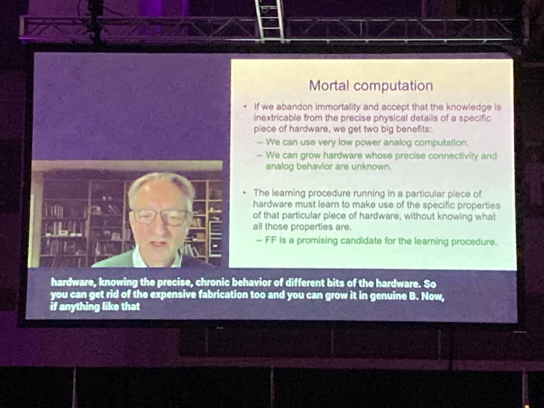
FF is the Best Learning Algorithm for Future Mortal Computers

Mortal Computation is one of Hinton’s recent important ideas (note: this term has not yet been officially translated into Chinese, temporarily translated as “非永生计算”).

He points out that current general-purpose digital computers are designed to faithfully follow instructions, and it is believed that the only way to make general-purpose computers perform specific tasks is to write a program that specifies in extremely detailed ways exactly what to do.

The mainstream idea remains to separate software from hardware, so the same program or the same set of weights can run on different physical copies of hardware. This leads to the knowledge contained in the program or weights becoming “immortal”: that is, when the hardware dies, the knowledge does not perish.

However, this is no longer valid, and the research community has not fully understood the long-term impact of deep learning on the construction of computers.

The separation of software and hardware is one of the foundations of computer science, which has indeed brought many benefits, such as allowing the properties of programs to be studied without having to worry about electrical engineering, and enabling the possibility of writing a program once and copying it to millions of computers. But Hinton points out:

If we are willing to give up this “immortality,” we can greatly save the energy required to perform computations and the cost of manufacturing hardware that executes computations.

In this way, different hardware instances performing the same task can vary significantly in connectivity and non-linearity, discovering effective parameter values that utilize the unknown properties of each specific instance from the learning process. These parameter values are only useful for specific hardware instances, so the computations they perform are not immortal but will perish with the hardware.

It makes no sense to copy parameter values to different hardware that operates differently, but we can transfer what one hardware has learned to another hardware in a more biological manner. For tasks like object classification in images, what we are truly interested in is the function that associates pixel intensities with class labels, rather than the parameter values that implement that function in specific hardware.

The function itself can be transferred to different hardware through distillation: training new hardware not only gives the same answers as the old hardware but also outputs the same probabilities for incorrect answers. These probabilities indicate more richly how the old model generalizes, rather than just the label it thinks is most likely. Therefore, by training the new model to match the probabilities of incorrect answers, we are training it to generalize in the same way as the old model. This kind of neural network training actually optimizes generalization, and this example is very rare.

If we want a trillion-parameter neural network to consume only a few watts, mortal computation may be the only choice. Its feasibility depends on whether we can find a learning process that can run efficiently on hardware with unknown precise details. In Hinton’s view, the FF algorithm is a promising candidate, though its performance in scaling to large neural networks remains to be observed.

At the end of the paper, Hinton pointed out the following unresolved questions:

Can FF generate sufficiently good image or video generative models to create the negative data needed for unsupervised learning?

If negative passes are completed during sleep, can positive and negative passes be temporally widely separated?

If the negative phase is eliminated for a period, does its effect resemble the destructive impact of severe sleep deprivation?

What goodness function works best? This paper uses the sum of squares of activities in most experiments, but minimizing the sum of squares of positive data activities and maximizing the sum of squares of negative data activities seems to work slightly better.

What activation function works best? Currently, only ReLU has been studied. Making activations the negative log density under t-distribution is one possibility.

For spatial data, can FF benefit from a large number of local optimization functions from different regions of the image? If feasible, it can accelerate the learning speed.

For sequential data, can fast weights be used to simulate simplified transformers?

Can a set of feature detectors trying to maximize their square activities and a set of constraint violation detectors trying to minimize their square activities support FF?