At the request of our backend team, this issue shares the practical implementation of Generative Adversarial Networks (GANs) using MATLAB. The content mainly includes a brief introduction to GAN and its classic variants, along with relevant code examples. If you want to learn more about deep learning, feel free to message me on the backend with your topics of interest; who knows, the next issue might cover what you want to learn!
1. Generative Adversarial Networks (GANs)
GAN consists of a generative model and a discriminative model. The task of the generative model is to generate instances that look naturally real and similar to the original data. The task of the discriminative model is to determine whether a given instance is real or artificially created. In fact, the principle of GAN can be metaphorically compared to a counterfeiting gang trying to produce and use counterfeit currency, while the discriminative model acts as the police detecting counterfeit money. The generator attempts to deceive the discriminator, and the discriminator strives not to be fooled by the generator. As the saying goes, ‘the higher the magic, the greater the skill.’ After multiple iterations of alternating optimization training, both models improve their performance, but what we need is a highly effective generative model (the counterfeiting gang) that produces results that are indistinguishable from real ones. The overall framework of GAN is shown in the figure below.
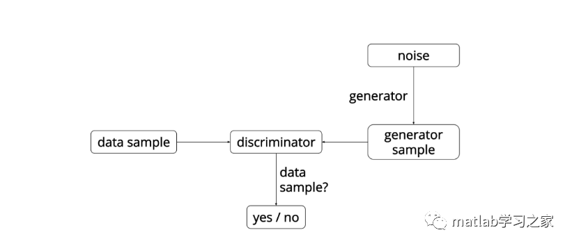
In practice, the generative network G generates images G(z) by accepting a random noise z, while the discriminator D needs to determine whether the input image x is real or not. The discriminator outputs the probability D(x) regarding the image’s authenticity; if the image is real, D(x) = 1, and if it is fake, D(x) = 0. During the iterative training process, the generator model attempts to generate realistic images to deceive the discriminator, while the discriminator tries to distinguish between generated images and real images, resulting in a dynamic game process. Ideally, the generator G is capable of producing images that are indistinguishable from real ones, making it difficult for the discriminator to determine the authenticity of images generated by G. Thus, D(G(z)) = 0.5.
The objective function of GAN is as follows:

Through continuous iterative training, GAN will eventually cause the data distribution of the images generated by the generator to approach that of the real data, as shown in the figure below.
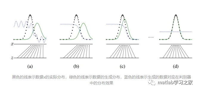
For the discriminator, if it receives a generated image, it should output 0; if it receives a real image, it should output 1, obtaining the error gradient for backpropagation to update parameters. For the generator, it first generates an image, then inputs it to the discriminator for judgment and obtains the corresponding error gradient, which is backpropagated to become the weights of the generator. Intuitively, this means that the discriminator must inform the generator how to adjust so that the images it generates become more realistic.
2. Variants of GAN
Due to certain issues with GAN itself, experts and scholars have proposed a series of variant algorithms, including DCGAN, LSGAN, SGAN, infoGAN, and others.
3. Practical Implementation of GAN in MATLAB
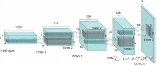
This time we share the practical implementation of DCGAN, which combines GAN with CNN, laying the foundation for almost all subsequent GAN architectures. DCGAN greatly enhances the stability of the original GAN training and the quality of the generated results. The framework of DCGAN is as follows:
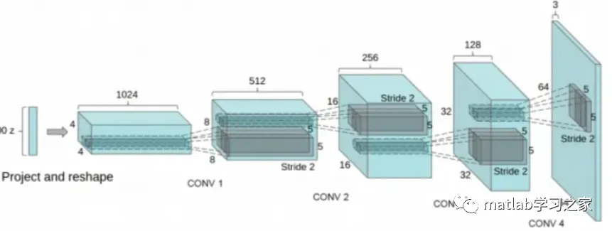
In the design of the DCGAN network, several popular improvements to CNN at that time were adopted:
1. Replacing the spatial pooling layer with convolutional layers. This replacement only requires setting the stride of the convolution to a value greater than 1. The significance of this improvement is that the downsampling process no longer discards certain pixel values at fixed positions but allows the network to learn the downsampling method itself.
2. Removing the fully connected layers.
3. Using Batch Normalization (BN), which is a normalization method commonly used after convolutional layers, helping the network converge.
4. Using Tanh (Sigmoid) activation function only in the output layer of the generator, while all other layers use ReLU activation function.
5. Using LeakyReLU activation function in all layers of the discriminator.
clear all; close all; clc;
%% Deep Convolutional Generative Adversarial Network
%% Load Data
load(‘mnistAll.mat’)
trainX = preprocess(mnist.train_images);
trainY = mnist.train_labels;
testX = preprocess(mnist.test_images);
testY = mnist.test_labels;
%% Settings
settings.latentDim = 100;
settings.batch_size = 32; settings.image_size = [28,28,1];
settings.lrD = 0.0002; settings.lrG = 0.0002; settings.beta1 = 0.5;
settings.beta2 = 0.999; settings.maxepochs = 50;
%% Generator
paramsGen.FCW1 = dlarray(initializeGaussian([128*7*7,…
settings.latentDim]));
paramsGen.FCb1 = dlarray(zeros(128*7*7,1,’single’));
paramsGen.TCW1 = dlarray(initializeGaussian([3,3,128,128]));
paramsGen.TCb1 = dlarray(zeros(128,1,’single’));
paramsGen.BNo1 = dlarray(zeros(128,1,’single’));
paramsGen.BNs1 = dlarray(ones(128,1,’single’));
paramsGen.TCW2 = dlarray(initializeGaussian([3,3,64,128]));
paramsGen.TCb2 = dlarray(zeros(64,1,’single’));
paramsGen.BNo2 = dlarray(zeros(64,1,’single’));
paramsGen.BNs2 = dlarray(ones(64,1,’single’));
paramsGen.CNW1 = dlarray(initializeGaussian([3,3,64,1]));
paramsGen.CNb1 = dlarray(zeros(1,1,’single’));
stGen.BN1 = []; stGen.BN2 = [];
%% Discriminator
paramsDis.CNW1 = dlarray(initializeGaussian([3,3,1,32]));
paramsDis.CNb1 = dlarray(zeros(32,1,’single’));
paramsDis.CNW2 = dlarray(initializeGaussian([3,3,32,64]));
paramsDis.CNb2 = dlarray(zeros(64,1,’single’));
paramsDis.BNo1 = dlarray(zeros(64,1,’single’));
paramsDis.BNs1 = dlarray(ones(64,1,’single’));
paramsDis.CNW3 = dlarray(initializeGaussian([3,3,64,128]));
paramsDis.CNb3 = dlarray(zeros(128,1,’single’));
paramsDis.BNo2 = dlarray(zeros(128,1,’single’));
paramsDis.BNs2 = dlarray(ones(128,1,’single’));
paramsDis.CNW4 = dlarray(initializeGaussian([3,3,128,256]));
paramsDis.CNb4 = dlarray(zeros(256,1,’single’));
paramsDis.BNo3 = dlarray(zeros(256,1,’single’));
paramsDis.BNs3 = dlarray(ones(256,1,’single’));
paramsDis.FCW1 = dlarray(initializeGaussian([1,256*4*4]));
paramsDis.FCb1 = dlarray(zeros(1,1,’single’));
stDis.BN1 = []; stDis.BN2 = []; stDis.BN3 = [];
% average Gradient and average Gradient squared holders
avgG.Dis = []; avgGS.Dis = []; avgG.Gen = []; avgGS.Gen = [];
%% Train
numIterations = floor(size(trainX,4)/settings.batch_size);
out = false; epoch = 0; global_iter = 0;
%% modelGradients
function [GradGen,GradDis,stGen,stDis]=modelGradients(x,z,paramsGen,…
paramsDis,stGen,stDis)
[fake_images,stGen] = Generator(z,paramsGen,stGen);
d_output_real = Discriminator(x,paramsDis,stDis);
[d_output_fake,stDis] = Discriminator(fake_images,paramsDis,stDis);
% Loss due to true or not
d_loss = -mean(.9*log(d_output_real+eps)+log(1-d_output_fake+eps));
g_loss = -mean(log(d_output_fake+eps));
% For each network, calculate the gradients with respect to the loss.
GradGen = dlgradient(g_loss,paramsGen,’RetainData’,true);
GradDis = dlgradient(d_loss,paramsDis);
end
%% progressplot
function progressplot(paramsGen,stGen,settings)
r = 5; c = 5;
noise = gpdl(randn([settings.latentDim,r*c]),’CB’);
gen_imgs = Generator(noise,paramsGen,stGen);
gen_imgs = reshape(gen_imgs,28,28,[]);
fig = gcf;
if ~isempty(fig.Children)
delete(fig.Children)
end
I = imtile(gatext(gen_imgs));
I = rescale(I);
imagesc(I)
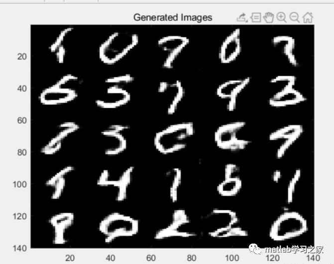
title(“Generated Images”)
colormap gray
drawnow;
end
%% dropout
function dly = dropout(dlx,p)
if nargin < 2
p = .3;
Experimental results are shown:
We hope everyone will submit more articles and show more support by liking and following!
Author | Hua Xia
Author | Hua Xia
Author | Hua Xia