1. Introduction
Generative Adversarial Networks (GAN) is a deep learning model framework proposed by Ian Goodfellow and his team in 2014, first published in the paper “Generative Adversarial Networks”.
Before the rise of deep learning, the main research directions for generative models included probabilistic graphical models (such as Hidden Markov Models (HMM)), variational inference methods (such as Variational Autoencoders (VAE)), and maximum likelihood estimation. However, these methods faced issues such as insufficient sample quality and training difficulties when generating complex data (such as images, audio, etc.).
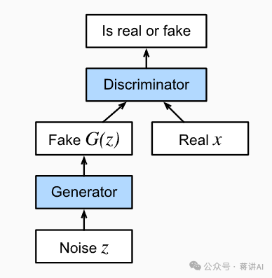
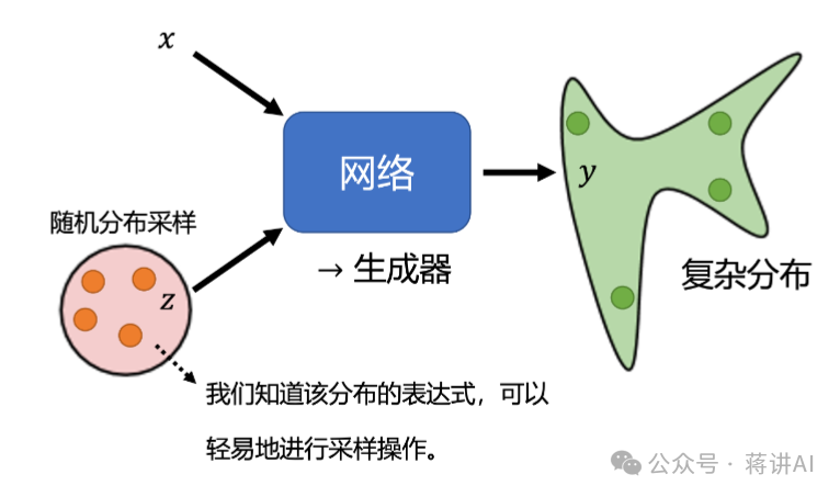
GAN introduces a game-theoretic framework, modeling the generative problem as a confrontation between two neural networks—Generator and Discriminator. The Generator takes random noise as input and generates samples that simulate the real data distribution, while the Discriminator attempts to distinguish between generated samples and real samples, as shown in the figure:
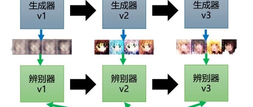
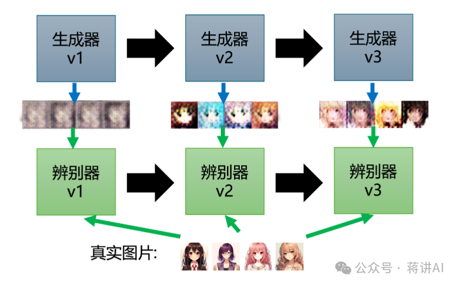
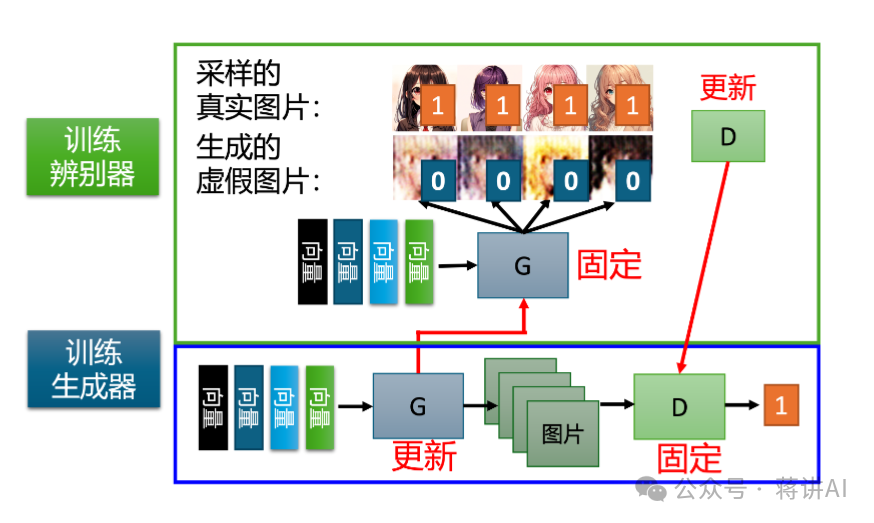
During the training process, the Generator and Discriminator confront each other. The Generator’s goal is to “deceive” the Discriminator, causing the generated samples to be classified as real data. The Discriminator’s goal is to improve its distinguishing ability to correctly identify generated samples and real data. Thus, the Generator and Discriminator maintain a continuous interactive and mutually reinforcing relationship, similar to what we call “involution”; they iteratively improve themselves to outsmart each other. Ultimately, the Generator learns to produce very realistic data samples, while the Discriminator learns to distinguish between real and generated data. Their training process is illustrated in the following figure:
The emergence of GAN marks a new stage in the research of generative models, becoming a significant milestone in the field of deep learning.
2. Principles
2.1 Discriminator
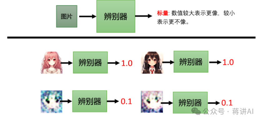
The job of the Discriminator is to distinguish whether the input data is real (from the real dataset) or generated (fake).
For the input data, the Discriminator outputs a value indicating the probability that it believes the data is real. The closer the value is to 1, the more the Discriminator “believes” it is real data; the closer the value is to 0, the more it “thinks” it is generated fake data. For example, in the task of generating anime avatars, the output of the Discriminator for real anime images would be 1, while the output for images generated by the Generator would be close to 0, as shown in the following figure:
The Discriminator is trained by minimizing a cross-entropy loss function:
Here, is the label, is the real data, and is the generated data. When , the loss function simplifies to:
To minimize this expression, for real data ( ), the Discriminator hopes that is as close to 1 as possible (i.e., very certain it is real data). If is small (discriminating incorrectly), the loss becomes larger, and the penalty increases.
When , the loss function simplifies to:
That is, for generated data ( ), the Discriminator hopes that is as close to 0 as possible (i.e., very certain it is generated data). If is large (discriminating incorrectly), the loss becomes larger, and the penalty increases.
This loss function essentially optimizes the Discriminator’s classification ability, enabling it to assign a higher value to real data (close to 1) and a lower value to generated data (close to 0). By minimizing this loss, the Discriminator gradually learns how to better distinguish between real and generated data.
2.2 Generator
The Generator receives a set of random noise (for example, random numbers sampled from a normal distribution or Gaussian distribution) and generates fake samples through a neural network. These generated samples belong to a complex distribution, as shown in the following figure, and the Generator itself will find ways to correspond this simple distribution to a more complex distribution:
The goal of the Generator is to “deceive” the Discriminator into believing that these fake samples are real. In other words, it hopes that . To achieve this goal, the Generator tries to maximize the Discriminator’s prediction error, using the following loss function during training:
This optimization method is more commonly used than the one proposed in the original paper as it avoids the problem of vanishing gradients. When is very small, gives a larger gradient signal, allowing the Generator’s gradients to be more stable, thus promoting the updates of the Generator.
Overall, the Discriminator and Generator confront each other, with the Discriminator striving to become smarter and not be deceived by the Generator, while the Generator works hard to produce more realistic data to deceive the Discriminator. The core objective of GAN can be summarized as a “min-max game”:
In other words, the Discriminator aims to minimize its loss by accurately distinguishing between real and fake. The Generator aims to maximize the Discriminator’s loss by generating data that is difficult for the Discriminator to distinguish.
Specifically:
Where the Discriminator’s objective is to minimize the loss for real data, i.e., . At the same time, it minimizes the judgment error for generated data, i.e., trying to reduce as much as possible. By optimizing these two parts, the Discriminator strives to bring close to 1 for real data and close to 0 for generated data. The Generator’s goal is to make it impossible for the Discriminator to distinguish between generated data and real data. It hopes that the output of generated data is as close to 1 as possible (i.e., classified as real data).
2.3 Training Process
The training process of the GAN algorithm can be divided into the following two main steps:
-
Fix the Generator and train the Discriminator: In this phase, the parameters of the Generator remain unchanged while optimizing the loss function of the Discriminator to enable it to more accurately distinguish between real data and the data generated by the Generator. The Discriminator gradually improves its ability to differentiate between real and fake data by minimizing its loss.
-
Fix the Discriminator and train the Generator: In this phase, the parameters of the Discriminator remain fixed while optimizing the loss function of the Generator to enable the generated data to deceive the Discriminator, i.e., to make the output of the Discriminator for the generated data close to the judgment result for real data.
The above two steps alternate. After training the Discriminator each time, the parameters of the Discriminator are fixed, switching to training the Generator; similarly, after completing the training of the Generator, it switches back to training the Discriminator. During the training process, the Generator continuously improves the distribution of generated data using feedback from the Discriminator, while the Discriminator continuously enhances its ability to distinguish between real data and generated data.
Through this alternating optimization approach, the Generator and Discriminator gradually approach an optimal state in their respective objectives, achieving a game equilibrium effect, as illustrated in the following figure:
3. Code Implementation
Here we present the code for the Deep Convolutional Generative Adversarial Network (DCGAN), which is an important variant of GAN that mainly improves the architecture of the Generator and Discriminator by introducing Convolutional Neural Networks (CNN) to enhance the performance and stability of the generative model. DCGAN belongs to the image generation type of GAN, specifically used for generating high-quality image data. Compared to the original GAN, DCGAN uses Convolutional Neural Networks instead of fully connected neural networks, making it more suitable for handling high-dimensional image data. The goal of this article is to generate anime faces, so the dataset consists entirely of anime faces.
The code is as follows (quoted from “Deep Learning by Li Hongyi”)
Dataset preparation:
# Download data from huggingface hub
!curl -s https://packagecloud.io/install/repositories/github/git-lfs/script.deb.sh | bash
!apt-get install git-lfs
!git lfs install
!git clone https://huggingface.co/datasets/LeoFeng/MLHW_6
!unzip ./MLHW_6/faces.zip -d .
GAN code implementation:
import os  # Python built-in library, provides operating system-related functions, such as file paths, environment variables, etc.
import glob  # Used for filename pattern matching, searching for path names that meet specific rules
import random  # Python built-in library, provides random number functionality
from datetime import datetime  # Python built-in library, used for obtaining or processing dates and times

import torch  # The main library of PyTorch, providing basic functions such as tensors and automatic differentiation
import torch.nn as nn  # PyTorch neural network module, includes definitions for network layers, loss functions, etc.
import torch.nn.functional as F  # Supplementary functions for various functions in nn, such as activation functions, etc.
import torchvision  # PyTorch's visual toolbox, including data preprocessing, models, image processing, etc.
import torchvision.transforms as transforms  # APIs related to image transformations in torchvision
from torch import optim  # Common optimizers in PyTorch, such as SGD, Adam, etc.
from torch.autograd import Variable  # Old-style writing, used to encapsulate tensors to support automatic differentiation (in the new version, Tensor is more commonly used)
from torch.utils.data import Dataset, DataLoader  # PyTorch dataset abstract class and data loading tool

import matplotlib.pyplot as plt  # Main plotting interface of the matplotlib plotting library
import numpy as np  # Python scientific computing library, supports multi-dimensional array operations
import logging  # Python built-in logging library, used for outputting and recording logs
from tqdm import tqdm  # Progress bar library, used for visualizing loop progress

# Set global random seed
def all_seed(seed = 6666):
    """
    Set random seed
    """
    np.random.seed(seed)  # Set numpy random seed
    random.seed(seed)  # Set random seed for the built-in random module in Python
    # CPU
    torch.manual_seed(seed)  # Set random seed for PyTorch on CPU
    # GPU
    if torch.cuda.is_available():  # If there is an available GPU
        torch.cuda.manual_seed_all(seed)  # Set seed for all available GPUs
        torch.cuda.manual_seed(seed)      # Set seed for the current default GPU
    # python global
    os.environ['PYTHONHASHSEED'] = str(seed)  # Set Python global environment variable to make random behavior controllable
    # cudnn
    torch.backends.cudnn.deterministic = True  # Use deterministic algorithms in convolution operations to ensure reproducible results
    torch.backends.cudnn.benchmark = False     # Disable cudnn's automatic search for the best algorithm
    torch.backends.cudnn.enabled = False       # Disable cudnn acceleration
    print(f'Set env random_seed = {seed}')  # Print the currently set random seed

all_seed(2022)  # Call the function to set the random seed to 2022
workspace_dir = '.'# Set the current working directory to the current folder

class CrypkoDataset(Dataset):
    def __init__(self, fnames, transform):
        self.transform = transform  # Save image transformation function
        self.fnames = fnames  # Save list of filenames
        self.num_samples = len(self.fnames)  # Record the number of samples in the dataset

    def __getitem__(self, idx):
        fname = self.fnames[idx]  # Get image file path based on index
        img = torchvision.io.read_image(fname)  # Read image as tensor (C,H,W)
        img = self.transform(img)  # Perform data preprocessing on the image (such as resize, normalize, etc.)
        return img  # Return processed image data

    def __len__(self):
        return self.num_samples  # Return dataset size

def get_dataset(root):
    fnames = glob.glob(os.path.join(root, '*'))  # Match all files in the root directory and return the path list
    compose = [
        transforms.ToPILImage(),  # Convert torch tensor to PIL image for subsequent operations
        transforms.Resize((64, 64)),  # Resize image to 64x64
        transforms.ToTensor(),  # Convert PIL image to torch tensor, pixel values from [0,255] -> [0,1]
        transforms.Normalize(mean=(0.5, 0.5, 0.5), std=(0.5, 0.5, 0.5)),  # Normalize: change [0,1] to [-1,1]
    ]
    transform = transforms.Compose(compose)  # Combine the above transformations into a whole transform
    dataset = CrypkoDataset(fnames, transform)  # Build a custom Dataset with these image filenames and transform
    return dataset  # Return the constructed Dataset

temp_dataset = get_dataset(os.path.join(workspace_dir, 'faces'))  # Get Dataset from './faces' path

images = [temp_dataset[i] for i in range(4)]  # Take the first 4 images from the dataset
grid_img = torchvision.utils.make_grid(images, nrow=4)  # Combine these 4 images into a grid
plt.figure(figsize=(10,10))  # Create a figure window of size 10x10
plt.imshow(grid_img.permute(1, 2, 0))  # permute changes (C,H,W) order to (H,W,C) for matplotlib display
plt.show()  # Show the image

# Generator
class Generator(nn.Module):  # Inherit from PyTorch's nn.Module, indicating a learnable network structure
    """
    Input shape: (batch, in_dim)
    Output shape: (batch, 3, 64, 64)
    """
    def __init__(self, in_dim, feature_dim=64):
        super(Generator, self).__init__()
        # The above two lines: call the parent class constructor and initialize the Generator class. in_dim is typically the dimension of the noise vector (e.g., 100).
        # feature_dim is the basic channel number of the Generator, which can control the channel size of intermediate layers in the network.

        # input: Input random one-dimensional vector (batch, 100)
        # Use linear layer + BN + ReLU to map the random vector to (batch, feature_dim*8*4*4)
        self.l1 = nn.Sequential(
            nn.Linear(in_dim, feature_dim * 8 * 4 * 4, bias=False),  # Fully connected layer: (batch, in_dim) -> (batch, feature_dim*8*4*4)
            nn.BatchNorm1d(feature_dim * 8 * 4 * 4),                 # Perform 1D batch normalization on the output of the linear layer
            nn.ReLU()                                               # ReLU activation
        )
        # Note: Reshape the output of l1 to (batch, feature_dim*8, 4, 4) and then perform upsampling convolution

        # l2 is a multi-layer transposed convolution network: changing channels from feature_dim*8 -> feature_dim*4 -> feature_dim*2 -> feature_dim
        # Corresponding spatial resolution upsampling from 4x4 to 32x32
        self.l2 = nn.Sequential(
            self.dconv_bn_relu(feature_dim * 8, feature_dim * 4),  # output -> (batch, feature_dim*4, 8, 8)
            self.dconv_bn_relu(feature_dim * 4, feature_dim * 2),  # output -> (batch, feature_dim*2, 16, 16)
            self.dconv_bn_relu(feature_dim * 2, feature_dim),      # output -> (batch, feature_dim, 32, 32)
        )

        # l3: Perform one more transposed convolution to upsample the resolution from 32x32 to 64x64 and output 3 channels (RGB)
        self.l3 = nn.Sequential(
            nn.ConvTranspose2d(feature_dim, 3, kernel_size=5, stride=2,
                               padding=2, output_padding=1, bias=False),
            nn.Tanh()  # Compress the generated image pixel range to [-1,1]
        )

        self.apply(weights_init)  # Apply custom weight initialization function

    def dconv_bn_relu(self, in_dim, out_dim):
        return nn.Sequential(
            nn.ConvTranspose2d(in_dim, out_dim, kernel_size=5, stride=2,
                               padding=2, output_padding=1, bias=False),  # Transposed convolution (deconvolution), performing spatial upsampling
            nn.BatchNorm2d(out_dim),  # 2D batch normalization
            nn.ReLU(True)            # ReLU activation
        )

    def forward(self, x):
        y = self.l1(x)                        # First use fully connected layer + BN + ReLU to transform (batch, in_dim) -> (batch, feature_dim*8*4*4)
        y = y.view(y.size(0), -1, 4, 4)       # reshape -> (batch, feature_dim*8, 4, 4)
        y = self.l2(y)                        # Pass through multiple layers of transposed convolution -> (batch, feature_dim, 32, 32)
        y = self.l3(y)                        # Final layer of transposed convolution -> (batch, 3, 64, 64), and use Tanh
        return y                              # Return the generated image


# Discriminator: Discriminator generates img and real img
class Discriminator(nn.Module):  # Inherit from nn.Module, indicating a learnable discriminator network
    """
    Input: (batch, 3, 64, 64)
    Output: (batch)
    """
    def __init__(self, in_dim, feature_dim=64):
        super(Discriminator, self).__init__()

        # input: (batch, 3, 64, 64)
        """
        In WGAN, the last layer sigmoid needs to be removed,
        Here is the standard GAN / DCGAN style, the last layer uses Sigmoid to output "real/fake" probabilities.
        """
        self.l1 = nn.Sequential(
            nn.Conv2d(in_dim, feature_dim, kernel_size=4, stride=2, padding=1), # First convolution layer -> (batch, 64, 32, 32)
            nn.LeakyReLU(0.2),                                                  # LeakyReLU activation
            self.conv_bn_lrelu(feature_dim, feature_dim * 2),                   # -> (batch, 128, 16, 16)
            self.conv_bn_lrelu(feature_dim * 2, feature_dim * 4),               # -> (batch, 256, 8, 8)
            self.conv_bn_lrelu(feature_dim * 4, feature_dim * 8),               # -> (batch, 512, 4, 4)
            nn.Conv2d(feature_dim * 8, 1, kernel_size=4, stride=1, padding=0),  # -> (batch, 1, 1, 1)
            nn.Sigmoid()                                                        # Map output to (0,1) interval
        )
        self.apply(weights_init)  # Apply weight initialization

    def conv_bn_lrelu(self, in_dim, out_dim):
        """
        In WGAN-GP, nn.Batchnorm cannot be used, and nn.InstanceNorm2d should be used instead.
        Here it is still DCGAN style, using BatchNorm2d.
        """
        return nn.Sequential(
            nn.Conv2d(in_dim, out_dim, 4, 2, 1),  # Convolution: kernel=4, stride=2, padding=1, reduce size by half
            nn.BatchNorm2d(out_dim),             # Batch normalization
            nn.LeakyReLU(0.2)                    # LeakyReLU activation
        )

    def forward(self, x):
        y = self.l1(x)  # Sequentially pass through the Discriminator layers, output dimension (batch, 1, 1, 1)
        y = y.view(-1)  # reshape -> (batch), each sample gets a scalar prediction
        return y        # Return the prediction score of the Discriminator for the input (usually interpreted as "real/fake probability")

# Network weight initialization
def weights_init(m):
    classname = m.__class__.__name__  # Get the current module class name to identify whether the layer is Conv or BatchNorm
    if classname.find('Conv') != -1:
        m.weight.data.normal_(0.0, 0.02)  # If it is a convolution layer, randomly initialize its weights from a normal distribution with mean 0 and standard deviation 0.02
    elif classname.find('BatchNorm') != -1:
        m.weight.data.normal_(1.0, 0.02)  # If it is a batch normalization layer, randomly initialize its weights from a normal distribution with mean 1 and standard deviation 0.02
        m.bias.data.fill_(0)             # Also initialize the bias of the batch normalization layer to 0


class TrainerGAN():
    def __init__(self, config):
        self.config = config                       # Save configuration, such as learning rate lr, batch_size, z_dim, etc.

        self.G = Generator(100)                    # Instantiate the Generator, input dimension defaults to 100
        self.D = Discriminator(3)                  # Instantiate the Discriminator, input channel number is 3 (RGB images)

        self.loss = nn.BCELoss()                   # Define binary cross-entropy loss for distinguishing real/fake samples

        """
        Note on optimizer settings:
            GAN: Use Adam optimizer
            WGAN: Use RMSprop optimizer
            WGAN-GP: Use Adam optimizer
        """
        # Set Adam optimizer for the Discriminator, using the learning rate config["lr"], Beta=(0.5, 0.999) is an empirical value for DCGAN
        self.opt_D = torch.optim.Adam(self.D.parameters(), lr=self.config["lr"], betas=(0.5, 0.999))
        # Set Adam optimizer for the Generator
        self.opt_G = torch.optim.Adam(self.G.parameters(), lr=self.config["lr"], betas=(0.5, 0.999))

        self.dataloader = None                      # Placeholder for loading data later
        self.log_dir = os.path.join(self.config["workspace_dir"], 'logs')         # Log directory
        self.ckpt_dir = os.path.join(self.config["workspace_dir"], 'checkpoints') # Model save directory

        # Log format setting
        FORMAT = '%(asctime)s - %(levelname)s: %(message)s'
        logging.basicConfig(level=logging.INFO,
                            format=FORMAT,
                            datefmt='%Y-%m-%d %H:%M')

        self.steps = 0                                                   # Used to record iteration steps
        self.z_samples = Variable(torch.randn(100, self.config["z_dim"])).cuda()
        # Pre-define some random noise z for visualizing the output of the Generator after each epoch

    def prepare_environment(self):
        """
        Prepare environment, data, and model before training
        """
        os.makedirs(self.log_dir, exist_ok=True)  # Create log directory (automatically create if not exists)
        os.makedirs(self.ckpt_dir, exist_ok=True) # Create ckpt directory (automatically create if not exists)

        # Update the naming of log and ckpt folders based on the current timestamp for distinguishing different training times
        time = datetime.now().strftime('%Y-%m-%d_%H-%M-%S')
        self.log_dir = os.path.join(self.log_dir, time+f'_{self.config["model_type"]}')
        self.ckpt_dir = os.path.join(self.ckpt_dir, time+f'_{self.config["model_type"]}')
        os.makedirs(self.log_dir)
        os.makedirs(self.ckpt_dir)

        # Data preparation: create dataloader
        dataset = get_dataset(os.path.join(self.config["workspace_dir"], 'faces'))  # Load image dataset from specified directory
        self.dataloader = DataLoader(dataset, batch_size=self.config["batch_size"],
                                     shuffle=True, num_workers=2)  # Create DataLoader to batch-read data

        # Model preparation
        self.G = self.G.cuda()  # Move Generator to GPU
        self.D = self.D.cuda()  # Move Discriminator to GPU
        self.G.train()          # Set Generator to train mode
        self.D.train()          # Set Discriminator to train mode

    def gp(self):
        """
        Implement gradient penalty function (empty implementation here, needed for WGAN-GP)
        """
        pass

    def train(self):
        """
        Train Generator and Discriminator
        """
        self.prepare_environment()  # Prepare training environment, data, model

        for e, epoch in enumerate(range(self.config["n_epoch"])):  # Train for n_epoch rounds
            progress_bar = tqdm(self.dataloader)                   # Use tqdm to display progress bar
            progress_bar.set_description(f"Epoch {e+1}")           # Add identifier to the progress bar

            for i, data in enumerate(progress_bar):
                imgs = data.cuda()                   # Get real images and move to GPU
                bs = imgs.size(0)                    # Number of samples in the current batch

                # *********************
                # *    Train D-Discriminator  *
                # *********************
                z = Variable(torch.randn(bs, self.config["z_dim"])).cuda()  # Generate random noise z
                r_imgs = Variable(imgs).cuda()                              # Actual images
                # The Generator generates fake photos
                f_imgs = self.G(z)                                         # Forward pass to generate fake images

                r_label = torch.ones((bs)).cuda()  # Label the real images as 1
                f_label = torch.zeros((bs)).cuda() # Label the fake images as 0

                # Forward pass through the Discriminator to get scores for real and fake images
                r_logit = self.D(r_imgs)
                f_logit = self.D(f_imgs)

                """
                DISCRIMINATOR loss setting note:
                    GAN:  loss_D = (r_loss + f_loss)/2
                    WGAN: loss_D = -torch.mean(r_logit) + torch.mean(f_logit)
                    WGAN-GP:
                        gradient_penalty = self.gp(r_imgs, f_imgs)
                        loss_D = -torch.mean(r_logit) + torch.mean(f_logit) + gradient_penalty
                """
                # Here we use the log loss (BCE) of the normal GAN: hoping the Discriminator can distinguish real images from fake images
                r_loss = self.loss(r_logit, r_label)  # BCE loss between real images and label 1
                f_loss = self.loss(f_logit, f_label)  # BCE loss between fake images and label 0
                loss_D = (r_loss + f_loss) / 2        # Overall loss of the Discriminator, taking the average

                # Backpropagation for the Discriminator
                self.D.zero_grad()    # Clear gradients of the Discriminator
                loss_D.backward()     # Backpropagation
                self.opt_D.step()     # Update parameters of the Discriminator

                """
                SET WEIGHT CLIP NOTE:
                    WGAN: Use the following code
                    for p in self.D.parameters():
                        p.data.clamp_(-self.config["clip_value"], self.config["clip_value"])
                """
                # The above segment is only needed in WGAN, and is commented out here

                # *********************
                # *    Train G-Generator  *
                # *********************
                # According to config["n_critic"], only update the Generator every n_critic steps
                if self.steps % self.config["n_critic"] == 0:
                    # Regenerate some fake photos
                    z = Variable(torch.randn(bs, self.config["z_dim"])).cuda()
                    f_imgs = self.G(z)

                    # Use the Discriminator to score these fake images
                    f_logit = self.D(f_imgs)

                    """
                    Generator loss function setting note:
                        GAN: loss_G = self.loss(f_logit, r_label)
                        WGAN: loss_G = -torch.mean(self.D(f_imgs))
                        WGAN-GP: loss_G = -torch.mean(self.D(f_imgs))
                    """
                    # In normal GAN, the goal of the Generator is to make the Discriminator classify the fake images as real (1), so use r_label=1
                    loss_G = self.loss(f_logit, r_label)

                    # Backpropagation for the Generator
                    self.G.zero_grad()
                    loss_G.backward()
                    self.opt_G.step()

                # Update loss information displayed on the progress bar
                if self.steps % 10 == 0:
                    progress_bar.set_postfix(loss_G=loss_G.item(), loss_D=loss_D.item())
                self.steps += 1

            # At the end of each epoch, use eval mode to generate some image samples for visualization
            self.G.eval()
            f_imgs_sample = (self.G(self.z_samples).data + 1) / 2.0  # Generate image pixel range [-1,1] -> [0,1]
            filename = os.path.join(self.log_dir, f'Epoch_{epoch+1:03d}.jpg')
            torchvision.utils.save_image(f_imgs_sample, filename, nrow=10)  # Save grid-like images

            logging.info(f'Save some samples to {filename}.')

            # Display images in notebook or script
            grid_img = torchvision.utils.make_grid(f_imgs_sample.cpu(), nrow=10)
            plt.figure(figsize=(10,10))
            plt.imshow(grid_img.permute(1, 2, 0))
            plt.show()

            self.G.train()  # Switch back to training mode

            # Save checkpoints for the Generator and Discriminator every 5 epochs (or at epoch 0)
            if (e+1) % 5 == 0 or e == 0:
                torch.save(self.G.state_dict(), os.path.join(self.ckpt_dir, f'G_{e}.pth'))
                torch.save(self.D.state_dict(), os.path.join(self.ckpt_dir, f'D_{e}.pth'))

        logging.info('Finish training')  # Print log after all training is complete

    def inference(self, G_path, n_generate=1000, n_output=30, show=False):
        """
        1. G_path: Path to the Generator model parameters
        2. n_generate: How many images to generate
        3. n_output: Only want to visualize how many in the notebook
        4. show: Whether to visualize and display
        """
        self.G.load_state_dict(torch.load(G_path))  # Load weights of the Generator
        self.G.cuda()
        self.G.eval()
        z = Variable(torch.randn(n_generate, self.config["z_dim"])).cuda()  # Generate random noise
        imgs = (self.G(z).data + 1) / 2.0  # Map generated results to [0,1]

        os.makedirs('output', exist_ok=True)  # Create output directory to save generated results
        for i in range(n_generate):
            torchvision.utils.save_image(imgs[i], f'output/{i+1}.jpg')  # Save each image individually

        if show:
            # If show=True, display some of them
            row, col = n_output // 10 + 1, 10
            grid_img = torchvision.utils.make_grid(imgs[:n_output].cpu(), nrow=row)
            plt.figure(figsize=(row, col))
            plt.imshow(grid_img.permute(1, 2, 0))
            plt.show()

config = {
    "model_type": "GAN",         # Model type, using original/classic GAN (i.e., DCGAN style)
    "batch_size": 64,            # Number of samples used in one training session
    "lr": 1e-3,                  # Learning rate, set to 0.001
    "n_epoch": 10,               # Total number of training rounds
    "n_critic": 1,               # Number of times the Discriminator (critic) updates before training the Generator once
    "z_dim": 100,                # Dimension of the noise vector input to the Generator
    "workspace_dir": workspace_dir,
}

trainer = TrainerGAN(config)     # Initialize TrainerGAN with the above config
trainer.train()                  # Start training
The running environment is as follows:
matplotlib                3.5.1
numpy                     1.21.5
python                    3.8.19
pytorch                   2.4.0
pytorch-cuda              12.1
torch                     1.12.0
tqdm                      4.66.5
We ran for 10 epochs on this dataset, and the final results are shown in the figure:
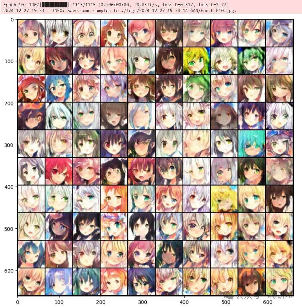
From the sampling results of 10 epochs, it can be seen that GAN has learned to generate anime faces with uniform styles and clear features, with overall quality significantly better than meaningless outputs from random noise. Although some images still exhibit slight overlaps and unnatural colors, the overall contours, hair colors, and expressions are already quite realistic, indicating that the model has converged to a certain extent, with acceptable diversity and stability in the generated samples. If training rounds are further increased or parameters adjusted, it is expected to achieve even more realistic synthetic samples.
In summary, the GAN network enables the Generator and Discriminator to engage in adversarial training: the Generator continuously learns to produce more realistic samples, while the Discriminator strives to distinguish between real and fake, resulting in mutual progress. It demonstrates powerful capabilities in fields such as image generation, speech synthesis, and data augmentation. However, GAN still faces challenges such as unstable training, mode collapse, and lack of controllability. Future development directions include improving training methods (such as WGAN-GP, StyleGAN, etc.), enhancing generation quality and controllability (introducing conditional generation, text-to-image, etc.), and further expanding application scenarios with the help of large models and multimodal technologies.