Click on the above “Beginner Learning Visuals“, choose to add “Star” or “Pin“
Heavyweight content delivered first timeImage
1. Analog Image
An analog image, also known as a continuous image, refers to an image that continuously changes in a two-dimensional coordinate system, meaning the pixels of the image are infinitely dense and have grayscale values (the variation of the image from dark to bright).
2. Digital Image
A digital image, also known as a digital image or bitmap image, is a representation of a two-dimensional image using a finite number of pixel values.
A digital image is obtained by digitizing an analog image, consisting of pixels as the basic element, which can be stored and processed by digital computers or digital circuits.
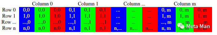
A typical two-dimensional digital image is a matrix, which can be represented by a two-dimensional array f(x,y), where x and y are coordinates in a two-dimensional spatial coordinate system, and f(x,y) represents the grayscale value and other properties of the image at that point.
3. Color Models (Color Storage)
Color has three characteristics: hue, brightness, and saturation. The three characteristics of color and their interrelationships can be illustrated using a three-dimensional color space model.
A color model is a model that represents a certain color in digital form, or a method of recording image colors. They include: RGB model, CMYK model, HSB model, Lab model, bitmap mode, grayscale mode, indexed color mode, duotone mode, and multi-channel mode.
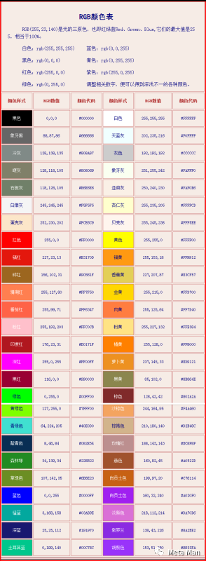
● RGB Model (Additive Color Model)
RGB is the most commonly used color model, where R, G, and B represent the three primary colors: red, green, and blue. In this model, each pixel occupies 3 bytes (one byte equals 8 bits), used to represent the R, G, and B components of the color (255, 255, 255) in the additive color model (black to white).
Characteristics include small file size and rich, vibrant colors. The RGB model is an additive color model. The images displayed on screens are generally in RGB mode, as the physical structure of monitors follows the RGB model.
When the brightness values of the three primary colors are equal, gray is produced; when all three brightness values are 255, pure white is produced; and when all brightness values are 0, pure black is produced. The method of color generation in the RGB model is also known as additive color mixing.
4. Color Modes (Display Methods)
Color modes are algorithms for representing colors in the digital world. In the mathematical world, to represent various colors, people usually divide colors into several components. Due to different principles of color generation, there are distinctions in the ways color devices like monitors, projectors, and scanners (which synthesize colors directly from light) and printing devices (which rely on pigments) generate colors. They are divided into: RGB model, CMYK model, HSB model, Lab model, bitmap mode, grayscale mode, indexed color mode, duotone mode, and multi-channel mode.
5. Types of Images
(1) Binary Image
Contains only black and white colors. Black is 0, and white is 1. Binary images are suitable for images composed of only black and white without grayscale shading.
(2) Grayscale Image (GrayScale)
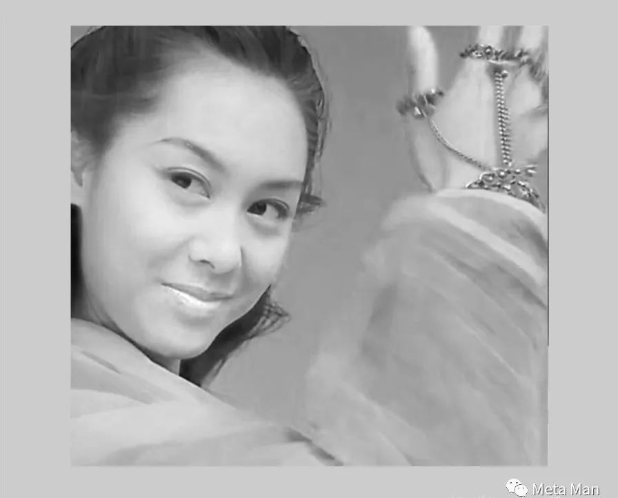
The value range of matrix elements in a grayscale image is typically [0, 255]. Therefore, its data type is generally an 8-bit unsigned integer (int8), which is commonly referred to as a 256 grayscale image. “0” represents pure black, “255” represents pure white, and the intermediate numbers represent the transition colors from black to white. Grayscale images contain only shades of gray and no color. What we usually refer to as black and white photos actually include all the grayscale tones between black and white.
(3) Indexed Color Image
The color table’s red, green, and blue component values are not all equal; pixel values are the index addresses of the image color table.
In this mode, the colors are pre-defined, and the available set of colors is limited; indexed color images can display a maximum of 256 colors.
Indexed colors are also referred to as mapped colors. An indexed color image is defined in the image file, and when the file is opened, the index values corresponding to the specific colors of the image are read into the program, which then finds the final colors based on the index values.
The file structure of indexed images is relatively complex, as it not only stores the two-dimensional matrix of the image but also includes a two-dimensional array known as the Color Index Matrix MAP. The size of the MAP is determined by the value range of the matrix elements; for example, if the matrix element value range is [0, 255], the size of the MAP matrix is 256×3, represented as MAP=[RGB]. Each row in the MAP specifies the red, green, and blue monochrome values corresponding to that row’s color, and each row corresponds to a grayscale value of the image matrix pixels.
The data type of indexed images is generally 8-bit unsigned integers (int8), and the corresponding index matrix MAP size is 256×3, so indexed images can only display a maximum of 256 colors simultaneously, but the types of colors can be adjusted by changing the index matrix.
Indexed images are generally used to store images with simpler color requirements, such as wallpapers in Windows, which often use indexed images; for images with more complex colors, true color RGB images are needed.
(4) True Color RGB Image
RGB images, like indexed images, represent the color of each pixel using combinations of red (R), green (G), and blue (B) primary colors.
However, unlike indexed images, the color values of each pixel in RGB images (represented by RGB primary colors) are stored directly in the image matrix. Since the color of each pixel is represented by the R, G, and B components, each component occupies 1 byte, representing different brightness values between 0 and 255, and the combination of these three bytes can produce 16.7 million different colors.
M and N represent the number of rows and columns of the image, and the three M x N two-dimensional matrices represent the R, G, and B color components of each pixel respectively. The data type of RGB images is generally 8-bit unsigned integers, typically used to represent and store true color images, but they can also store grayscale images.
RGB images are stored in rows and columns, with each column containing three channels (note: the order of channels is BGR instead of RGB).
5. Main Differences Between RGB Images and Indexed Images
(1) RGB Color Mode Image: Also known as additive mode image, it is the best color for screen display, composed of red, green, and blue colors, each of which can have brightness variations from 0 to 255.
(2) Indexed Color Image: In this color mode, image pixels are represented by one byte, and it can contain up to 256 colors stored in a color table, indexed by the colors used, resulting in lower image quality. Its data information includes a data matrix and a double precision color table matrix, where the values in the data matrix directly specify the color of that point as one from the color table matrix, with each row representing a color and three data points indicating the proportions of red, green, and blue in that color, with all element values within [0, 1]. It occupies less space and is commonly used for image transmission on the web, where strict requirements exist for image pixels and sizes.
6. Pixel
A pixel refers to a small square that makes up an image, each with a specific position and assigned color value. The color and position of these small squares determine how the image is presented. Digital images are composed of pixels, which are often categorized based on the position of the coordinate origin, with each pixel denoted as I(r,c) or f(x,y). The value range I of grayscale images is a scalar: I=greylevel; the value range I of color images is a vector: I=(r,g,b).
Pixels can be viewed as indivisible units or elements of the entire image. Indivisible means that they cannot be further divided into smaller units or elements; they exist as a small square of a single color.
Each raster image contains a certain number of pixels, which determine the size of the image as displayed on the screen.
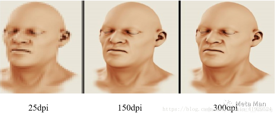
7. Resolution
Resolution is a parameter that measures the amount of data within a bitmap image. It is typically expressed in pixels per inch (PPI) and dots per inch (DPI).
(1) Image Resolution
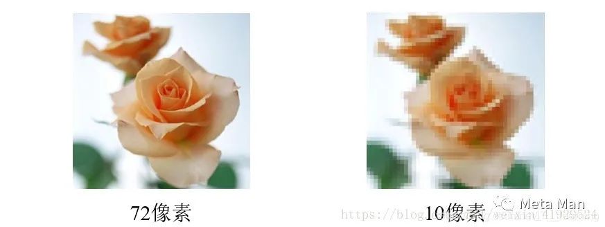
The number of pixels per unit length in an image is referred to as the image’s resolution, measured in pixels/inch (PPI) or pixels/cm. In two images of the same size, the high-resolution image contains more pixels than the low-resolution image.
The size of the image, the image resolution, and the image file size are closely related. The larger the image size, the higher the image resolution, and consequently, the larger the image file. Adjusting the image size and resolution can change the image file size.
(2) Screen Resolution
Screen resolution is the number of dots displayed per unit length on the monitor (DPI). Screen resolution depends on the size of the monitor and its pixel settings.
When the image resolution exceeds the monitor resolution, the images displayed on the screen appear larger than their actual size.
Mathematical Models of Images
1. Two Basic Mathematical Models of Images
Continuous Model
General images are a continuous distribution of energy, as in film imaging.
Discrete Model
This model views a digital image as a collection of discrete sampling points, each with its own attributes. Processing operations involve these discrete units. It cannot reflect the overall state of the image or the relationships between image contents. Convolution operations are better suited for this.
Both models have their advantages and disadvantages, but the future direction will still focus on the discrete model, as it is more convenient for computer processing, which will be the primary approach for image processing.
2. Principles of Application for Mathematical Models of Images
In image processing, different models are often used based on the tasks and objectives, or different models are used at different stages to ensure optimal system performance. Images must satisfy the sampling theorem during digitalization so that discrete images correspond to their continuous forms. “Digital image processing” refers not to “the processing of digital images” but to “the digital processing of images.”
3. Sampling Theorem
The sampling theorem, proposed by American telecommunications engineer H. Nyquist in 1928, serves as a fundamental bridge between continuous-time signals (commonly referred to as “analog signals”) and discrete-time signals (commonly referred to as “digital signals”) in the field of digital signal processing. The theorem describes the relationship between sampling frequency and signal spectrum, serving as the basic basis for the discretization of continuous signals. It establishes a sufficient condition for the sampling rate that allows discrete sampling sequences to capture all information from finite bandwidth continuous-time signals.
4. Digitalization (Continuous → Discrete)
The process of converting an image from its original form to a digital form involves three steps: “scanning” (scanning), “sampling” (sampling), and “quantization” (quantization). Usually, “scanning” is combined into the “sampling” phase, merging into two processes.

(1) Sampling
Sampling is the process of transforming a spatially continuous image into discrete points; the higher the sampling frequency, the more realistic the restored image.
Sampling divides a continuous image into M×N grids, each represented by a brightness value. Each grid is referred to as a pixel. The values of M and N must satisfy the sampling theorem.

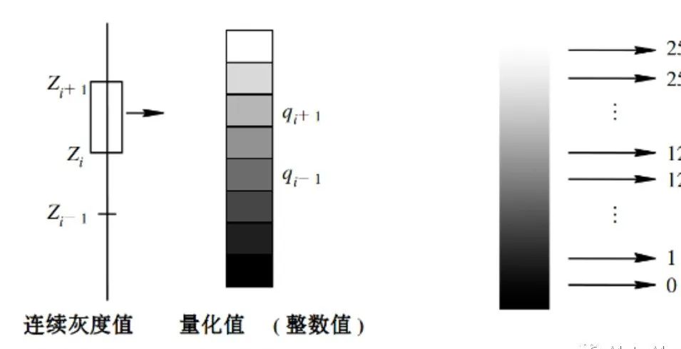
(2) Quantization
Quantization is the process of converting sampled pixel points into discrete numerical values. The number of different grayscale values in a digital image is referred to as grayscale levels; the higher the level, the clearer the image.
Quantization converts the continuous range of brightness values at the sampling points into a single specific numerical value.
After quantization, the image is represented as an integer matrix. Each pixel has two attributes: position and grayscale. The position is represented by rows and columns. The grayscale represents the integer indicating the brightness level at that pixel’s position. This numerical matrix M×N becomes the object for computer processing. Grayscale levels are typically between 0-255 (8-bit quantization). The following image illustrates how the continuous is transformed into discrete.
In summary, the digitalization process is illustrated below, representing the transition from the true source of the image to the final digital image:
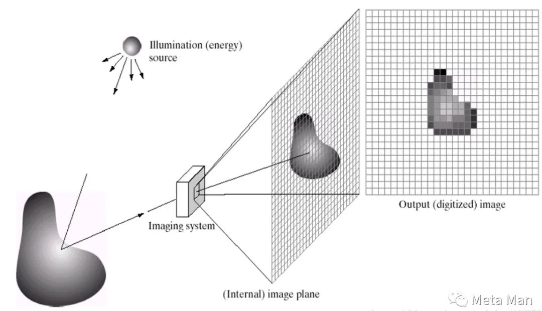
Image Processing
Digital image processing includes:
● Image digitization;
● Image transformation;
● Image enhancement;
● Image restoration;
● Image compression coding;
● Image segmentation;
● Image analysis and description;
● Image recognition and classification.
Common Image Transformation Algorithms
Geometric transformations of images (image distortion correction, image scaling: bilinear interpolation, rotation, stitching)
Image transformations (Fourier, cosine, Walsh-Hadamard, K-L transform, wavelet transform)
Image frequency domain processing (enhancement algorithms: high-frequency enhancement, homomorphic filtering; smoothing and denoising: low-pass filtering)
Image Enhancement
The purpose of image enhancement is to improve the visual effect of images, enhancing the overall or local characteristics of the image for specific applications, making previously unclear images clearer or enhancing certain features of interest, expanding the differences between various objects in the image, and suppressing uninteresting features to improve image quality and enrich information content, thus enhancing image interpretation and recognition effects to meet certain feature analysis needs.
Common image enhancement methods include linear transformations of images; nonlinear transformations of images; histogram equalization and specification of images.
Image Restoration
Images may degrade in quality due to imperfections in imaging systems, transmission media, and devices, a phenomenon known as image degradation. Image restoration requires prior knowledge of the mechanisms and processes of image degradation to find a corresponding inverse process calculation method to obtain the restored image. If an image has degraded, it should be restored before enhancement.
Common image restoration methods include:
● Algebraic restoration methods: unconstrained restoration; constrained least squares method
● Frequency domain restoration methods: inverse filtering restoration; removing blur caused by uniform motion; Wiener filtering restoration method
Image Compression
Image data can be compressed because there is redundancy in the data. In image compression, there are three basic types of data redundancy: coding redundancy; inter-pixel redundancy; visual redundancy.
● Lossless compression: This is a compression of the file itself, optimizing the data storage method of the file, using an algorithm to represent repeated data information, allowing the file to be fully restored without affecting the content. For digital images, it also does not result in any loss of image details. In lossless (also known as lossless, error-free, information-preserving) encoding, only redundant data in the image is deleted, and the reconstructed image after decoding is identical to the original image without any distortion.
● Lossy compression: This involves altering the image itself, retaining more brightness information while merging hue and saturation information with surrounding pixels, resulting in a high compression ratio due to reduced information volume, which will correspondingly lower image quality. Lossy (also known as lossy, distorted) encoding means that the reconstructed image after decoding differs from the original image, cannot be precisely restored, but visually appears similar, achieving a high compression ratio.
This article is for academic sharing only. If there is any infringement, please contact us to delete the article.
Good news! <br/>Beginner Learning Visual Knowledge Planet is now open to the public 👇👇👇<br/><br/>Download 1: OpenCV-Contrib Extension Module Chinese Version Tutorial<br/>Reply "Extension Module Chinese Tutorial" in the "Beginner Learning Visuals" WeChat account backend to download the first OpenCV extension module tutorial in Chinese available online, covering installation of extension modules, SFM algorithms, stereo vision, target tracking, biological vision, super-resolution processing, and more than twenty chapters of content.<br/><br/>Download 2: Python Visual Practical Projects 52 Lectures<br/>Reply "Python Visual Practical Projects" in the "Beginner Learning Visuals" WeChat account backend to download 31 visual practical projects, including image segmentation, mask detection, lane line detection, vehicle counting, eyeliner addition, license plate recognition, character recognition, emotion detection, text content extraction, and facial recognition, to help quickly learn computer vision.<br/><br/>Download 3: OpenCV Practical Projects 20 Lectures<br/>Reply "OpenCV Practical Projects 20 Lectures" in the "Beginner Learning Visuals" WeChat account backend to download 20 practical projects based on OpenCV for advanced learning of OpenCV.<br/><br/>Group Chat<br/><br/>Welcome to join the reader group of the WeChat account to communicate with peers. Currently, there are WeChat groups for SLAM, 3D vision, sensors, autonomous driving, computational photography, detection, segmentation, recognition, medical imaging, GAN, algorithm competitions, etc. (these will gradually be subdivided). Please scan the WeChat ID below to join the group, and note: "Nickname + School/Company + Research Direction", for example: "Zhang San + Shanghai Jiao Tong University + Visual SLAM". Please follow the format; otherwise, it will not be approved. After successful addition, you will be invited to relevant WeChat groups based on your research direction. Please do not send advertisements in the group; otherwise, you will be removed from the group. Thank you for your understanding~