
0 Introduction
Over the past few days, I have been watching some videos and reading blog posts about Convolutional Neural Networks (CNNs). I have organized the useful knowledge and content that I found helpful here, to clarify the logic and deepen my understanding. I can easily refer back to this in the future, ensuring it will never be lost.
1 Convolutional Neural Networks
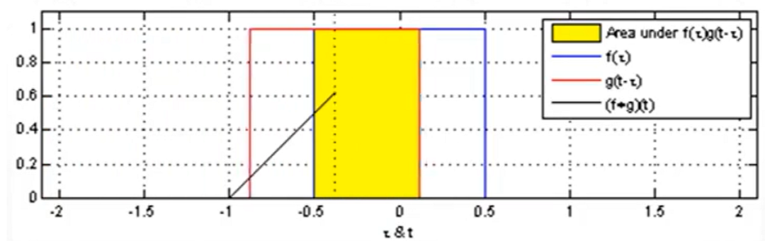
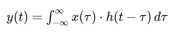
Since it is called a Convolutional Neural Network, the first part is convolution, and then there is neural network, which is a combination of the two. The concept of convolution actually comes from the field of signal processing, typically involving the convolution operation of two signals, as shown in the figure below:
|
|
|
|
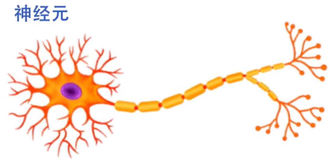
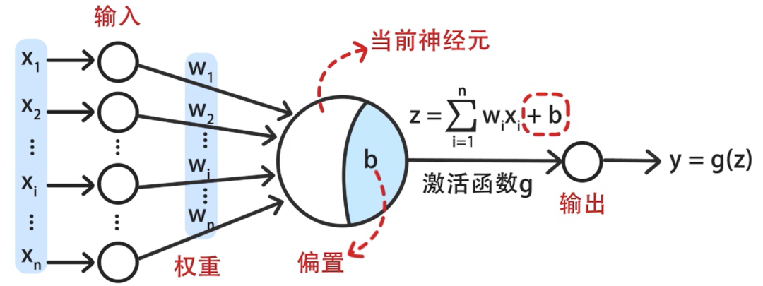
Neural Networks, this is a veteran of machine learning, simulating the working mechanism of human brain neurons. Each neuron is a computational unit that multiplies the input data by weights, sums it up, adds a bias, and then passes the result through an activation function to produce an output. As shown in the figure below, multiple neurons are interconnected to form a neural network, but I won’t elaborate on that here.
|
|
|
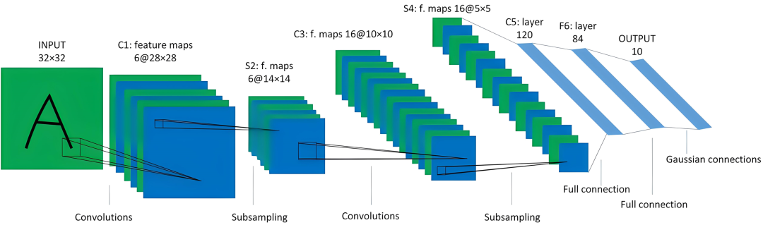
Convolutional Neural Networks have numerous applications in image classification and recognition, initially used for handwritten digit classification, and have gradually developed from there.
2 Image Formats
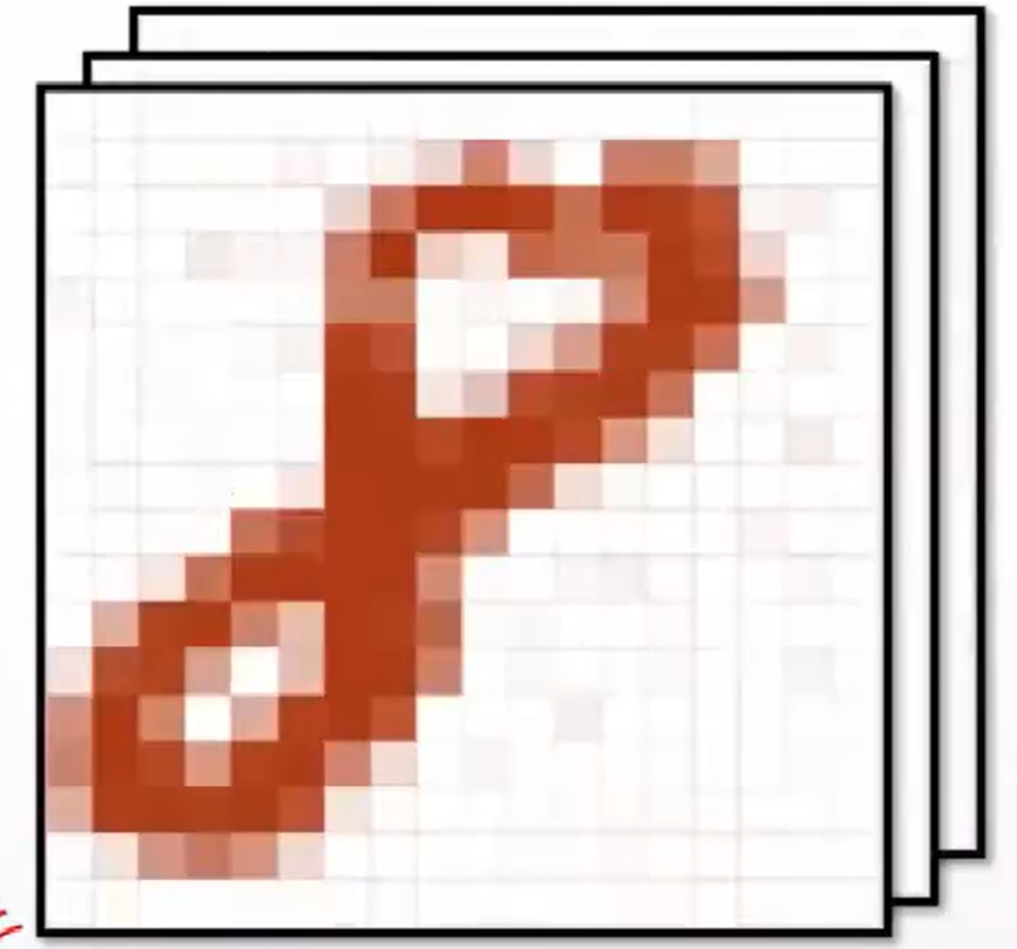
Let’s start with handwritten image recognition. If an image is monochrome, it can be viewed as a two-dimensional numerical matrix, where the color of each pixel can be represented by a grayscale value. If the image is colored, it can be considered as a combination of three monochrome images (RGB).
 |
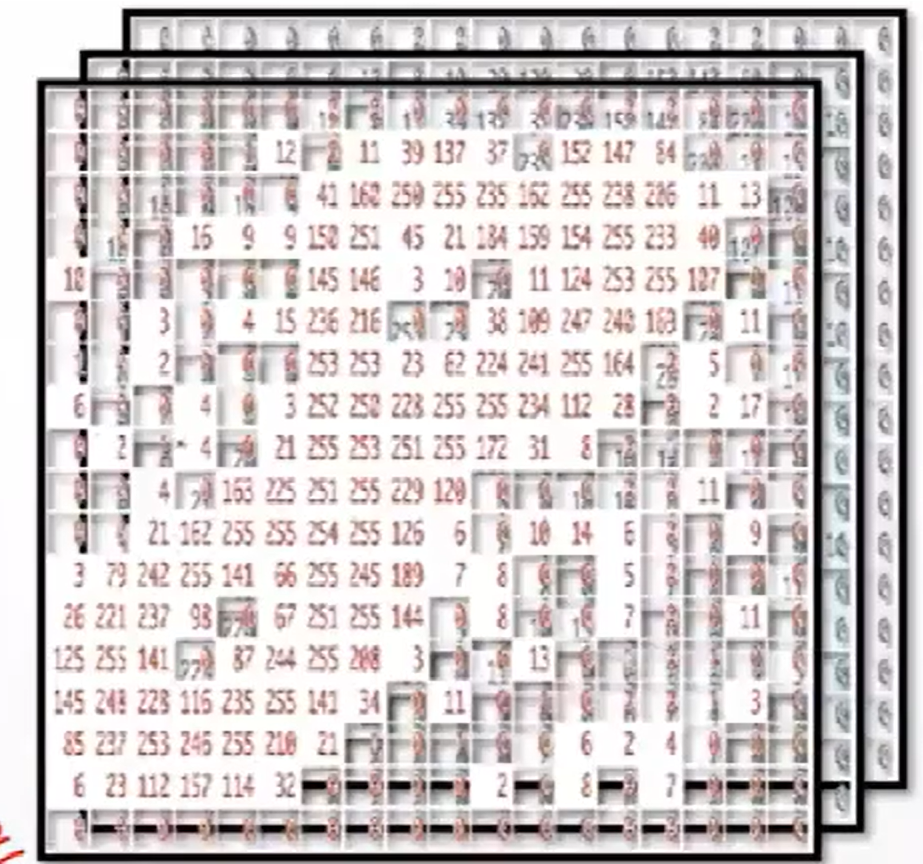 |
Each pixel in an image is actually a numerical value, and the whole image can be viewed as a three-dimensional matrix.
3 Image Convolution Operations
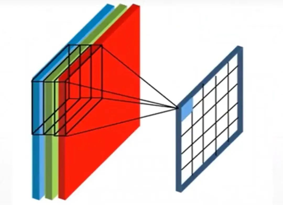
So what exactly happens when we perform convolution on a colored image? The animated image below illustrates the process of image convolution calculation well. The original image has three RGB channels (channel1-3), corresponding to three convolution kernels (Kernel1-3). Each channel’s image is subjected to a multiply-add operation with its corresponding convolution kernel. The values obtained from each channel are summed up, and after adding the overall bias, we get a value in the feature map.
The next image is a three-dimensional representation.
4 Kernels and Feature Maps
The first question here is why the convolution kernel is 3×3 in size. This dimension has been established through ongoing research by scholars, and it is currently believed that a 3×3 receptive field is sufficient, while also keeping the computational load relatively low. There are also 1×1 convolution kernels in use, while others are generally not used.
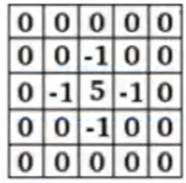
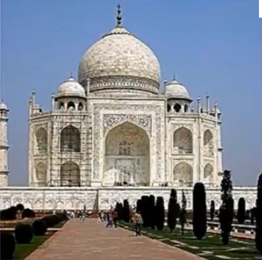
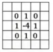
The second question is how the parameters in the convolution kernel are derived. These parameters are implemented through machine learning. Once we adjust all the kernel parameters, the model is determined. There are also some predefined convolution kernels, such as those below, which can achieve sharpening and edge detection effects after convolution.
|
|
|
|
|
|
|

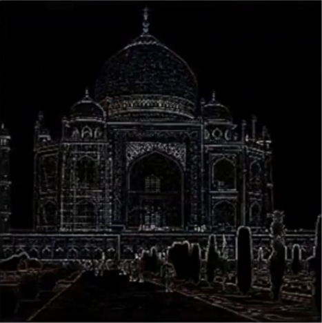
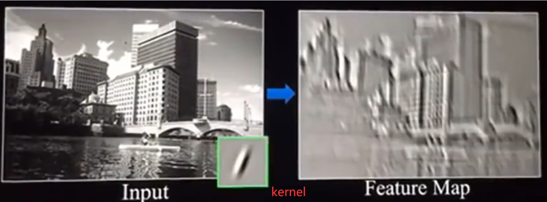
After performing convolution on an image, we obtain a feature map, which extracts some features. Using different kernels for convolution will output multiple feature maps.
Convolution kernels (Kernels) are also known as filters.
A feature map is the result obtained after the image pixel values are filtered.
The following two images visually demonstrate the actual appearance of kernels and feature maps.
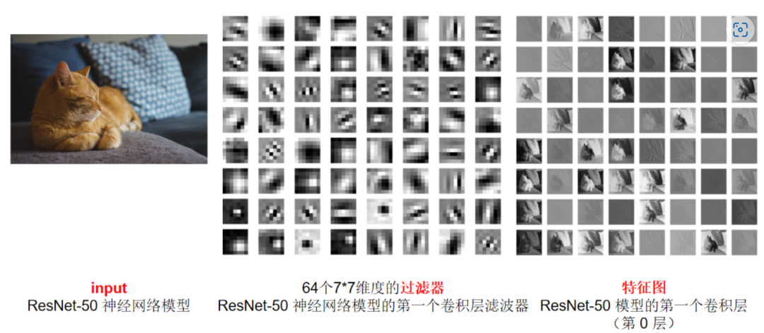
During the processing of Convolutional Neural Networks, as the model computations deepen, the image dimensions (h*w) will become smaller, but the extracted features will increase.
5 Padding
Due to boundary issues, after each convolution, the image will inevitably be compressed a little. This involves a concept called padding. If the padding value is set to “same“, a layer of pixels will be added around the original image, generally padding with zeros, so that the subsequent image dimensions will match the original image. The default parameter is “valid“, which means that the pixels of the image being operated on with the convolution kernel are all valid, essentially meaning there is no outer layer of zeros.
| unvalid |
|
valid |
|
The image below demonstrates the convolution effect with padding. The issue with this image is that it uses a 4×4 convolution kernel, which is not typically used in practice.
Using a 3×3 convolution kernel can keep the image size unchanged after convolution.
Image source: https://github.com/vdumoulin/conv_arithmetic
6 Stride/Stride
The above image shows the case where the stride is 1. If the stride is 2, it means that convolution is performed every two rows or columns, effectively reducing the dimensionality, resulting in a smaller feature map size after convolution.
Image source: https://github.com/vdumoulin/conv_arithmetic
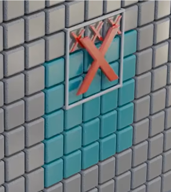
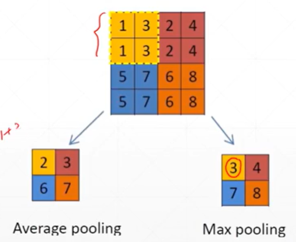
7 Pooling
Pooling mainly serves to reduce dimensionality and is also known as down-sampling, effectively avoiding overfitting. There are mainly two types of pooling methods: Max pooling and Avg pooling. Typically, the pooling area is 2×2 in size, so a 4×4 image will become 2×2 after pooling.
8 Shape
In TensorFlow and PyTorch, the structure of shapes differs.
TensorFlow input shape is (batch_size, height, width, in_channels) / (number of samples, image height, image width, number of image channels)
PyTorch input shape is (batch_size, in_channels, height, width)
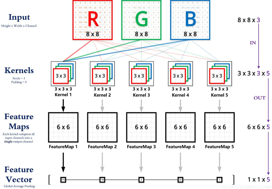
In the above image,
Input image shape: [inChannels, height, width] / [3, 8, 8];
Convolution kernel shape: [outChannels, inChannels, height, width] / [5, 3, 3, 3];
Output image shape: [outChannels, outHeight, outWidth] / [5, 6, 6];
The number of input channels for the convolution kernel (in depth) is determined by the number of channels in the input matrix (inChannels). For example, an RGB formatted image has an input channel count of 3.
The number of output channels in the output matrix (out depth) is determined by the output channel count of the convolution kernel. For example, in the animation below, if the convolution kernel has 8, then the output outChannels will be 8.
Image source: https://animatedai.github.io/
9 Epoch, Batch, Batch Size, Step
Epoch: represents the training process where all samples in the training dataset are passed through once (and only once). In one epoch, the training algorithm will sequentially input all samples into the model for forward propagation, loss calculation, backward propagation, and parameter updates. An epoch usually contains multiple steps.
Batch:Generally translated as “batch”, it represents a group of samples input to the model at one time. During the training process of neural networks, the training data is often large, such as tens of thousands or even hundreds of thousands of entries. If we input all this data at once, it would place too high a demand on computer performance and the learning capacity of the neural network model. Therefore, the training data can be divided into multiple batches, and each batch of samples can be input together into the model for forward propagation, loss calculation, backward propagation, and parameter updates. However, it should be noted that the term batch is not often used; in most cases, people focus on the batch size.
Batch Size (Batch Size): indicates the number of images passed to the model in a single training session. During neural network training, we often need to divide the training data into multiple batches; the specific number of samples in each batch is determined by the batch size.
Step:Generally translated as “step”, it represents the operation of updating parameters in a model once during an epoch. In simple terms, completing the training of a batch of data corresponds to completing a step.
10 Neural Networks
In fact, the convolution processing above is all about feature extraction from images, and to perform classification or prediction, we need to rely on neural networks. Therefore, after convolution processing, the data usually needs to be flattened to become one-dimensional, making it easier to input into the input layer of the neural network.
In a neural network model (see the image below), the fully connected layer/Dense layer is a commonly used type of neural network layer in deep learning, also known as a dense connection layer or multilayer perceptron layer. It can serve as an input layer (input layer), output layer (output layer), or hidden layer (Hidden layer).
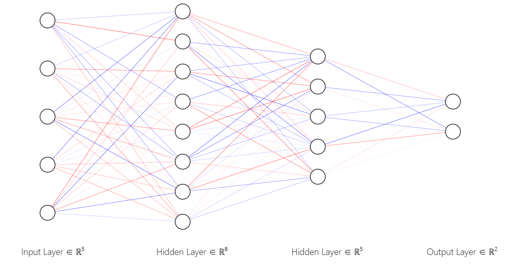
Recommended tool for drawing neural network diagrams: NN-SVG.
11 Activation Functions
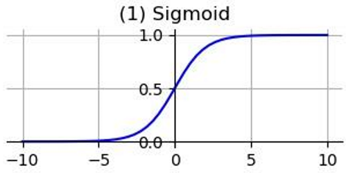
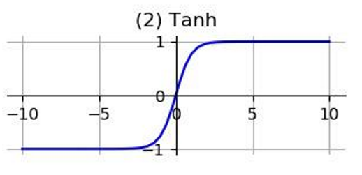
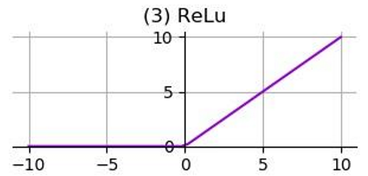
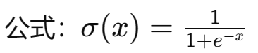
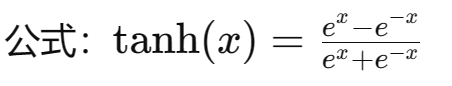
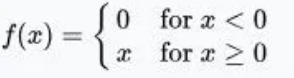
In neural networks, activation functions are used to introduce non-linearity, allowing the network to learn complex mapping relationships. If activation functions are not used, each layer’s output will be a linear function of the upper layer’s input. Regardless of how many layers the neural network has, the output will be a linear combination of the input. Here are some commonly used activation functions:
|
|
|
|
|
|
|
|
That’s all for now.