Exploring Pre-Trained Neural Networks for Feature Extraction

Introduction

In this article, I will explore a common practice in representation learning—using the frozen states of pre-trained neural networks as feature extractors.

Specifically, I am interested in comparing the performance of simple models trained using these extracted neural network features with that of fine-tuned neural networks initialized with transfer learning. The intended audience is primarily data scientists and anyone interested in computer vision and machine learning.

A little ahead… The results below indicate that the performance of scikit-learn models trained with extracted neural network features is nearly comparable to that of the complete networks fine-tuned with the same pre-trained weights (the balanced accuracy drops by 3% to 6%).

Background

Today, companies like Microsoft release thousands of pre-trained neural network models every year. These models are becoming increasingly powerful and easier to use.

With so many model checkpoints open-sourced, the evolution of neural networks as a core focus in artificial intelligence/machine learning is not surprising. Think of the DALL-E-2 and Stable Diffusion neural networks that can convert text prompts into images/artworks.

Reportedly, Stable Diffusion has been downloaded by over 10 million users. What many do not realize is that these technologies exist today largely due to advancements in the statistical subfield of representation learning.

“The 2020s look like the era when representation learning realizes its promise in machine learning. By using models trained on specific domains (supervised or unsupervised), we can use their later activations as representations of their inputs when processing inputs.

Representations can be used in various ways, most commonly as direct inputs to downstream models or as targets for co-training shared latent spaces with multiple model types (text and vision, GNN and text, etc.).”—Kyle Kranen[1]

Let’s examine these claims…

Dataset Details

The image dataset used below is sourced from the Chesapeake Conservancy land cover project from 2013/2014[2].

It consists of National Agriculture Imagery Program (NAIP) satellite images providing four information channels (red, green, blue, and near-infrared) at a resolution of 1 meter square. The original geospatial data spans six states, covering a total area of 100,000 square miles: Virginia, West Virginia, Maryland, Delaware, Pennsylvania, and New York.

To obtain n = 15,809 unique patches of size 128 x 128 pixels and the same number of land cover labels, it was first subsampled. Examining the example patches (see Figure 1), the 1-meter square resolution appears quite detailed, as structures and objects in the images can be interpreted with considerable clarity.

Note: The original Chesapeake Conservancy land cover dataset includes label masks intended for segmentation rather than classification. To change this, I only kept patches that appeared with a single class and occurred at least 85% of the time when sampling the geospatial data.

Here, the five land cover categories used in the experiments are defined as follows:

• Water: Open water bodies including ponds, rivers, and lakes

• Canopy and Shrubs: Woody plants including trees and shrubs

• Low Vegetation: Plant material with a height of less than 2 meters, including lawns

• Barren: Natural soil areas without growing vegetation

• Impervious Surfaces: Man-made surfaces

Upon inspection, the dataset appears to have many interesting features, including seasonal variations (e.g., foliage), noise, and distribution shifts across the six states. A small amount of “natural” noise helps make this somewhat simplified classification task more challenging, which is beneficial, as we do not want the supervised task to be too easy.

Using states as a partitioning mechanism, training, validation, and test sets were generated. The test set selected patches from Pennsylvania (n=2,586, accounting for 16.4% of the data), the validation set selected patches from Delaware (n=2,088, accounting for 13.2% of the data), and the remainder was used for the training set (n=11,135, accounting for 70.4% of the data).

Overall, the dataset has a significant class imbalance problem: barren land (49/15,809) and impervious surfaces (124/15,809) are underrepresented, while canopy and shrubs (9,514/15,809) are overrepresented. In contrast, low vegetation (3,672/15,809) and water (2,450/15,809) are more balanced.

Due to label imbalance, we use balanced accuracy in the experiments below. This metric averages the individual accuracies of each class as a statistic, giving equal weight to each class regardless of its size.

see: torchgeo.datasets

Learning Features

Typically, learning features can be defined as features derived from black box algorithms. By extracting image representations as learning features, you typically trust other teams in the computer vision community who have optimized the algorithms when initially training the black box.

For example, packages like keras, pytorch, and transformers can be used to extract learning features from neural networks pre-trained on large benchmark datasets like ImageNet.

Learning features are often excellent representations for downstream tasks, whether unsupervised or supervised. The assumption made is that the model’s weights have been pre-trained in a robust manner. Fortunately, you can trust Google / Microsoft / Facebook on this.

To provide some context, when the original image is input into the neural network, it undergoes several consecutive transformation layers, where each hidden state layer extracts new information from the original image. After inputting the image into the network, the hidden states or embeddings can be directly extracted as features. The common practice is to use the last hidden state embedding as the extracted feature, i.e., the layer before the preceding supervised task head.

In this project, we will examine two pre-trained models: Microsoft’s Bidirectional Encoder Image Transformer (BEiT)[3] and Facebook’s ConvNext model[4].

BEiT-base and ConvNext-base are two of the most popular checkpoints for image classification on Hugging Face, performing well in preliminary tests and outperforming other options. Since the extracted hidden states are often higher than the 1 x n dimensions, a common practice is to average along the smaller dimension to obtain a 1 x n embedding for each image.

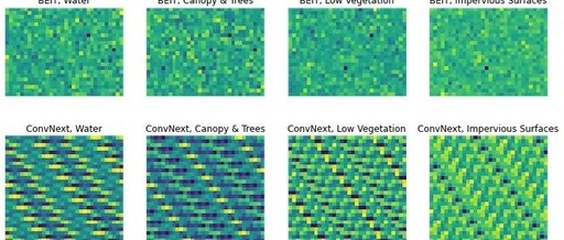
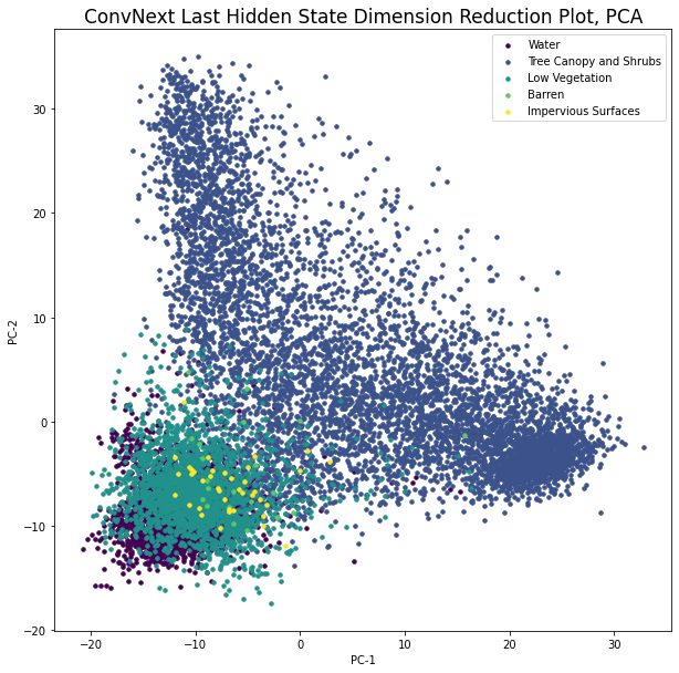
Below, we obtained a 1 x 768 embedding from the base BEiT and a 1 x 1024 dimensional embedding from the base ConvNext. These embeddings were arbitrarily reshaped into rectangular shapes for visualization, revealing some different patterns.

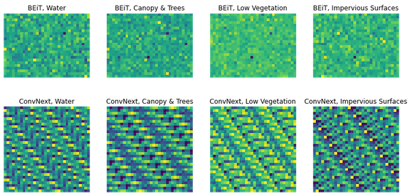
Figure 2 shows two learning feature representations of four random examples from the dataset. The top row corresponds to the BEiT Vision Transformer embeddings, while the bottom row corresponds to the ConvNext model embeddings. The four patches are from Water (left), Tree Canopy and Shrubs (left middle), Low Vegetation (right middle), and Impervious Surfaces (right). Note that these embeddings have been resized from the original 1 x n embeddings to visualize them as rectangular patches.

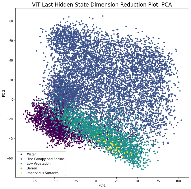
Next, we will look at how the data is visually presented in the learning feature space. To do this, we will perform PCA on n image embeddings to transform them into 2D space. Then we will plot them with class labels as colors.

see: transformers.BeitModel/ConvNextModel

Modeling

If you go to Kaggle competition notebooks, you will find that using pre-trained neural networks for transfer learning and fine-tuning is currently the most common practice in image classification.

In this case, the weights are first loaded into the network (transfer learning), and then updated on a new dataset of interest (fine-tuning). The latter step is typically run over several epochs and uses smaller learning weights so as not to deviate too far from the original weights.

However, compared to using the same model as a feature extractor, the transfer learning and fine-tuning process typically requires more time and computation.

The first half of the models below is trained using learning features and scikit-learn models. I used the following packages to implement the complete process: from feature extraction (transformers) to model training (sklearn) to hyperparameter optimization (optuna).

For hyperparameter optimization, I searched various logistic regressors and feedforward neural networks (FFNN) in 10 random trials, with results showing that an FFNN with a hidden state of dimension 175-200 is typically the best choice.

The transfer learning and fine-tuned neural networks were then trained to compare with these learning feature models, constituting the second part of the models. I used the transformers package to fine-tune the BEiT and ConvNext base models, which are entirely the same as the models above. For better comparison, the same pre-trained weights were used.

See Hugging Face’s excellent image classification tutorial: https://colab.research.google.com/github/nateraw/huggingface-hub-examples/blob/main/vit_image_classification_explained.ipynb

see: optuna, sklearn, transformers

Model Evaluation

To evaluate the models, I chose to check balanced accuracy, accuracy for each class, and the confusion matrix on the held-out test set. The confusion matrix shows where the model makes mistakes, helping to explain. Each row represents known samples present in a given class (actual values), while each column represents samples classified by the model (predicted values). The sum of each row equals the number of actual values present, while the sum of each column equals the number of predicted values.

Model 1, BEiT embeddings + sklearn FFNN:

Balanced accuracy… 79.6%

+============+=======+========+============+========+=========+
|            | Water | Trees  | Vegetation | Barren | Manmade |
+============+=======+========+============+========+=========+
| Water      |    64 |      0 |          2 |      0 |       0 |
+------------+-------+--------+------------+--------+---------+
| Trees      |     1 |   1987 |          3 |      1 |       0 |
+------------+-------+--------+------------+--------+---------+
| Vegetation |     1 |      3 |        457 |      0 |       0 |
+------------+-------+--------+------------+--------+---------+
| Barren     |     2 |      0 |         14 |      5 |       3 |
+------------+-------+--------+------------+--------+---------+
| Manmade    |     0 |      0 |          6 |      2 |      35 |
+------------+-------+--------+------------+--------+---------+

Accuracy for each class… Water: 97.0%, Tree Canopy and Shrubs: 99.7%, Low Vegetation: 99.1%, Barren: 20.8%, Impervious Surfaces: 81.4%.

The Beit embeddings model performed third overall.

Model 2, ConvNext embeddings + sklearn FFNN:

Balanced accuracy… 78.1%

+============+=======+========+============+========+=========+
|            | Water | Trees  | Vegetation | Barren | Manmade |
+============+=======+========+============+========+=========+
| Water      |    62 |      0 |          4 |      0 |       0 |
+------------+-------+--------+------------+--------+---------+
| Trees      |     2 |   1982 |          6 |      2 |       0 |
+------------+-------+--------+------------+--------+---------+
| Vegetation |     1 |      3 |        457 |      0 |       0 |
+------------+-------+--------+------------+--------+---------+
| Barren     |     1 |      1 |         17 |      4 |       1 |
+------------+-------+--------+------------+--------+---------+
| Manmade    |     0 |      0 |          8 |      0 |      35 |
+------------+-------+--------+------------+--------+---------+

Classification accuracy… Water: 93.9%, Tree Canopy and Shrubs: 99.5%, Low Vegetation: 99.1%, Barren: 16.6%, Impervious Surfaces: 81.4%.

The ConvNext embeddings model performed the worst overall.

Model 3, Fine-tuned BEiT neural network:

Balanced accuracy… 82.9%

+============+=======+========+============+========+=========+
|            | Water | Trees  | Vegetation | Barren | Manmade |
+============+=======+========+============+========+=========+
| Water      |    64 |      0 |          2 |      0 |       0 |
+------------+-------+--------+------------+--------+---------+
| Trees      |     0 |   1986 |          5 |      1 |       0 |
+------------+-------+--------+------------+--------+---------+
| Vegetation |     2 |      3 |        455 |      0 |       1 |
+------------+-------+--------+------------+--------+---------+
| Barren     |     0 |      0 |         13 |      9 |       2 |
+------------+-------+--------+------------+--------+---------+
| Manmade    |     1 |      0 |          6 |      1 |      35 |
+------------+-------+--------+------------+--------+---------+

Classification accuracy… Water: 97.0%, Tree Canopy and Shrubs: 99.7%, Low Vegetation: 98.7%, Barren: 37.5%, Impervious Surfaces: 81.4%.

The fine-tuned BEiT model ranked second overall.

Model 4, Fine-tuned ConvNext neural network:

Balanced accuracy… 84.4%

+============+=======+========+============+========+=========+
|            | Water | Trees  | Vegetation | Barren | Manmade |
+============+=======+========+============+========+=========+
| Water      |    65 |      0 |          1 |      0 |       0 |
+------------+-------+--------+------------+--------+---------+
| Trees      |     0 |   1978 |         12 |      2 |       0 |
+------------+-------+--------+------------+--------+---------+
| Vegetation |     1 |      2 |        457 |      0 |       1 |
+------------+-------+--------+------------+--------+---------+
| Barren     |     0 |      0 |         13 |     11 |       0 |
+------------+-------+--------+------------+--------+---------+
| Manmade    |     0 |      0 |          7 |      2 |      34 |
+------------+-------+--------+------------+--------+---------+

Classification accuracy… Water: 98.5%, Tree Canopy and Shrubs: 99.3%, Low Vegetation: 99.1%, Barren: 45.8%, Impervious Surfaces: 79.1%.

The fine-tuned ConvNext model performed the best overall.

Improvements/Limitations in the Modeling Process:

The modeling process can be improved in multiple ways, including those discussed next. These models performed the worst in classifying barren land, so if I could make a single change, I would first add more of this type of classification.

Currently, these models are effectively more like 4 classifiers, as the performance on barren land is very poor. Another improvement would be to use cross-validation in hyperparameter optimization; however, cross-validation requires longer run times and may be a bit excessive for this experiment.

The generalization limitations of the output models include poorer performance on images of other class types, different resolutions, and other conditions (new objects, new structures, new classes, etc.). I have pushed the fine-tuned ConvNext and BEiT to Hugging Face for hosted inference, where the models can be tested for generalization performance by loading images and/or running defaults configured in each model.

Lessons Learned

1. Mastering Python packages is crucial. See the code blocks in this article listing the various libraries used.

2. Visualizing changes in image features can provide deeper insights into the signals in the dataset.

3. Pre-trained embeddings combined with simpler models can perform almost as well as fine-tuned neural networks.

4. Hugging Face excels not only in natural language processing but also in computer vision!

Conclusion:

What do these results and learnings imply for neural networks in today’s computer vision field? Let’s review.

In 2017, Andrej Karpathy, the former head of Tesla’s Autopilot division, discussed the shift from traditional engineering to deep learning in a famous blog post, which he referred to as “Software 2.0”[5].

From this perspective, neural networks are not “just another tool in the machine learning toolbox.” Instead, they represent a shift in how we can develop software.

Thank you for reading!

References

[1] K. Kranen (2022), The 2020s are looking like the age of representation learning’s promise being realized in ML, LinkedIn.

[2] Chesapeake Bay Program Office (2022). One-meter Resolution Land Cover Dataset for the Chesapeake Bay Watershed, 2017/18. Developed by the University of Vermont Spatial Analysis Lab, Chesapeake Conservancy, and U.S. Geological Survey. [Nov 15, 2022], [URL],

• Dataset License: The dataset used herein is publicly available to all without restriction.

[3] Bao, H., Dong, L., & Wei, F. (2021). BEiT: BERT Pre-Training of Image Transformers. CoRR, abs/2106.08254. https://arxiv.org/abs/2106.08254

[4] Liu, Z., Mao, H., Wu, C.-Y., Feichtenhofer, C., Darrell, T., & Xie, S. (2022). A ConvNet for the 2020s. CoRR, abs/2201.03545. https://arxiv.org/abs/2201.03545

[5] A. Karpathy (2017), Software 2.0, Medium.

[6] Nanni, L., Ghidoni, S., & Brahnam, S. (2017). Handcrafted vs. non-handcrafted features for computer vision classification. Pattern Recognition, 71, 158–172. doi:10.1016/j.patcog.2017.05.025

Appendix

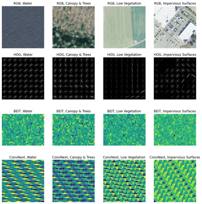
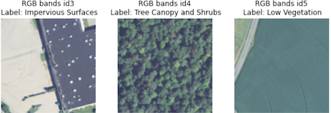
In computer vision, non-learning features can be considered handcrafted features from images[6]. The optimal non-learning features for a given problem often rely on understanding the location of different signals in the dataset. Before extracting non-learning features, let’s plot some random image patches in RGB space.

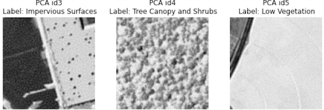
We will first explore Principal Component Analysis (PCA) as the first non-learning feature. PCA is a dimensionality reduction technique, and we use it here to convert 128 x 128 x 4 images into 1 x n vectors. The size n of the PCA transformed dataset is user-specified and can be any number less than the original dimensions of the data.

Internally, the algorithm uses feature vectors (the extended directions in the data) and eigenvalues (the relative importance of the directions) to find a basis that retains the maximum variance from the original images. Once the calculations are complete, PCA can be used to transform new images into lower-dimensional space and/or visualize the images in two or three dimensions (see Figures 3 and 4).

In the example below, when n = 3000, the PCA results retain 95% of the dimensions and preserve nearly all signals from the original images. To visualize PCA, I reversed the operation and plotted the examples as 128 x 128 pixel images.

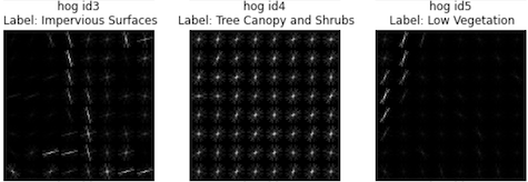
Let’s take a look at another old-school feature: Histogram of Oriented Gradients (HOG). To compute HOG, gradients (intensity of change) and directions are first calculated on the image. Then the image is divided into several cells, where the directions are layered into histogram bins. Then, at each pixel in the cell, we look for its direction, find the corresponding bin in the histogram, and add the given value to it. This process is then repeated across the image’s cells. Done!

Check out the cool performance of HOG here:

While these handcrafted features are interesting as a first tool for visualizing the dataset, they are not suitable for our supervised modeling purposes. Here, initial tests indicate that models built using HOG and PCA features have significantly lower balanced accuracy compared to models trained with the learning features discussed below (PCA dropped by 35%, HOG dropped by 50%).

see: skimage.feature.hog, sklearn.decomposition.PCA