

This article is approximately 4000 words, and it is recommended to read in 10minutes
A time series refers to any quantifiable measurement or event that occurs over a period of time. Although this may sound trivial, almost anything can be considered a time series. Your average heart rate per hour over a month, the daily closing price of a stock over a year, the number of traffic accidents in a city per week over a year. Recording this information over any period of time is considered a time series. For each of these examples, there is a frequency of events (daily, weekly, hourly, etc.) and a duration of time for the events (a month, a year, a day, etc.).

Our goal is to receive a sequence of values and predict the next value in that sequence. The simplest method is to use an autoregressive model, and we will focus on using LSTM to solve this problem.
Data Preparation
Let’s look at a sample time series. The figure below shows some data on oil prices from 2013 to 2018.
This is just a graph of a single numerical sequence on a date axis. The table below shows the first 10 entries of this time series. There is price data every day.
date dcoilwtico 2013-01-01 NaN 2013-01-02 93.14 2013-01-03 92.97 2013-01-04 93.12 2013-01-07 93.20 2013-01-08 93.21 2013-01-09 93.08 2013-01-10 93.81 2013-01-11 93.60 2013-01-14 94.27Many machine learning models perform much better on standardized data. The standard method for standardizing data is to transform the data so that the mean of each column is 0 and the standard deviation is 1. Below is the code using scikit-learn for standardization:
 from sklearn.preprocessing import StandardScaler
 # Fit scalers scalers = {} for x in df.columns:   scalers[x] = StandardScaler().fit(df[x].values.reshape(-1, 1))
 # Transform data via scalers norm_df = df.copy() for i, key in enumerate(scalers.keys()):   norm = scalers[key].transform(norm_df.iloc[:, i].values.reshape(-1, 1))   norm_df.iloc[:, i] = norm
We also want the data to have a uniform frequency— in this case, we have daily oil prices over these 5 years. If your data does not have this, Pandas has several different methods to resample data to fit a uniform frequency; please refer to previous articles on our public account.
For the training data, we need to slice the complete time series data into fixed-length sequences. Suppose we have a sequence: [1, 2, 3, 4, 5, 6].
By selecting a sequence of length 3, we can generate the following sequences and their associated targets:
[Sequence] Target
[1, 2, 3] → 4
[2, 3, 4] → 5
[3, 4, 5] → 6
In other words, we define how many steps back we need to look to predict the next value. We call this value the training window, and the number of values to predict is called the prediction window. In this example, they are 3 and 1, respectively. The following function details how this is done.
 # Defining a function that creates sequences and targets as shown above
def generate_sequences(df: pd.DataFrame, tw: int, pw: int, target_columns, drop_targets=False):
    '''
    df: Pandas DataFrame of the univariate time-series
    tw: Training Window - Integer defining how many steps to look back
    pw: Prediction Window - Integer defining how many steps forward to predict
    returns: dictionary of sequences and targets for all sequences
    '''
    data = dict()  # Store results into a dictionary
    L = len(df)
    for i in range(L-tw):  # Option to drop target from dataframe
        if drop_targets:
            df.drop(target_columns, axis=1, inplace=True)
        # Get current sequence
        sequence = df[i:i+tw].values
        # Get values right after the current sequence
        target = df[i+tw:i+tw+pw][target_columns].values
        data[i] = {'sequence': sequence, 'target': target}
    return data
This way we can use the Dataset class in PyTorch to customize our dataset.
 class SequenceDataset(Dataset):
    def __init__(self, df):
        self.data = df
    def __getitem__(self, idx):
        sample = self.data[idx]
        return torch.Tensor(sample['sequence']), torch.Tensor(sample['target'])
    def __len__(self):
        return len(self.data)
Then, we can use PyTorch DataLoader to iterate through the data. The benefit of using DataLoader is that it automatically batches and shuffles the data internally, so we don’t have to implement it ourselves. The code is as follows:
 # Here we are defining properties for our model
 BATCH_SIZE = 16  # Training batch size
 split = 0.8  # Train/Test Split ratio
 sequences = generate_sequences(norm_df.dcoilwtico.to_frame(), sequence_len, nout, 'dcoilwtico')
 dataset = SequenceDataset(sequences)
 # Split the data according to our split ratio and load each subset into a
 # separate DataLoader object
 train_len = int(len(dataset)*split)
 lens = [train_len, len(dataset)-train_len]
 train_ds, test_ds = random_split(dataset, lens)
 trainloader = DataLoader(train_ds, batch_size=BATCH_SIZE, shuffle=True, drop_last=True)
 testloader = DataLoader(test_ds, batch_size=BATCH_SIZE, shuffle=True, drop_last=True)
In each iteration, the DataLoader will produce 16 (batch size) sequences and their associated targets, which we will pass to the model.
Model Architecture
We will use a single LSTM layer, followed by some linear layers for the regression part of the model, with dropout layers in between. This model will output a single value for each training input.
 class LSTMForecaster(nn.Module):

    def __init__(self, n_features, n_hidden, n_outputs, sequence_len, n_lstm_layers=1, n_deep_layers=10, use_cuda=False, dropout=0.2):
        '''
        n_features: number of input features (1 for univariate forecasting)
        n_hidden: number of neurons in each hidden layer
        n_outputs: number of outputs to predict for each training example
        n_deep_layers: number of hidden dense layers after the lstm layer
        sequence_len: number of steps to look back at for prediction
        dropout: float (0 < dropout < 1) dropout ratio between dense layers
        '''
        super().__init__()
        self.n_lstm_layers = n_lstm_layers
        self.nhid = n_hidden
        self.use_cuda = use_cuda  # set option for device selection
        # LSTM Layer
        self.lstm = nn.LSTM(n_features,
                            n_hidden,
                            num_layers=n_lstm_layers,
                            batch_first=True)
        # As we have transformed our data in this way
        # first dense after lstm
        self.fc1 = nn.Linear(n_hidden * sequence_len, n_hidden)  # Dropout layer
        self.dropout = nn.Dropout(p=dropout)
        # Create fully connected layers (n_hidden x n_deep_layers)
        dnn_layers = []
        for i in range(n_deep_layers):
            # Last layer (n_hidden x n_outputs)
            if i == n_deep_layers - 1:
                dnn_layers.append(nn.ReLU())
                dnn_layers.append(nn.Linear(nhid, n_outputs))
            # All other layers (n_hidden x n_hidden) with dropout option
            else:
                dnn_layers.append(nn.ReLU())
                dnn_layers.append(nn.Linear(nhid, nhid))
                if dropout:
                    dnn_layers.append(nn.Dropout(p=dropout))
        # compile DNN layers
        self.dnn = nn.Sequential(*dnn_layers)
    def forward(self, x):
        # Initialize hidden state
        hidden_state = torch.zeros(self.n_lstm_layers, x.shape[0], self.nhid)
        cell_state = torch.zeros(self.n_lstm_layers, x.shape[0], self.nhid)
        # move hidden state to device
        if self.use_cuda:
            hidden_state = hidden_state.to(device)
            cell_state = cell_state.to(device)
        self.hidden = (hidden_state, cell_state)
        # Forward Pass
        x, h = self.lstm(x, self.hidden)  # LSTM
        x = self.dropout(x.contiguous().view(x.shape[0], -1))  # Flatten lstm out
        x = self.fc1(x)  # First Dense
        return self.dnn(x)  # Pass forward through fully connected DNN.
We have set two parameters that can be freely tuned: n_hidden and n_deep_layers. Larger parameters mean a more complex model and longer training times, so we can flexibly adjust these two parameters here.
The remaining parameters are as follows: sequence_len refers to the training window, and nout defines how many steps to predict; setting sequence_len to 180 and nout to 1 means the model will look at the situation 180 days (half a year) later to predict what will happen tomorrow.
 nhid = 50  # Number of nodes in the hidden layer
 n_dnn_layers = 5  # Number of hidden fully connected layers
 nout = 1  # Prediction Window
 sequence_len = 180  # Training Window
 # Number of features (since this is a univariate timeseries we'll set
 # this to 1 -- multivariate analysis is coming in the future)
 ninp = 1
 # Device selection (CPU | GPU)
 USE_CUDA = torch.cuda.is_available()
 device = 'cuda' if USE_CUDA else 'cpu'
 # Initialize the model
 model = LSTMForecaster(ninp, nhid, nout, sequence_len, n_deep_layers=n_dnn_layers, use_cuda=USE_CUDA).to(device)
Model Training
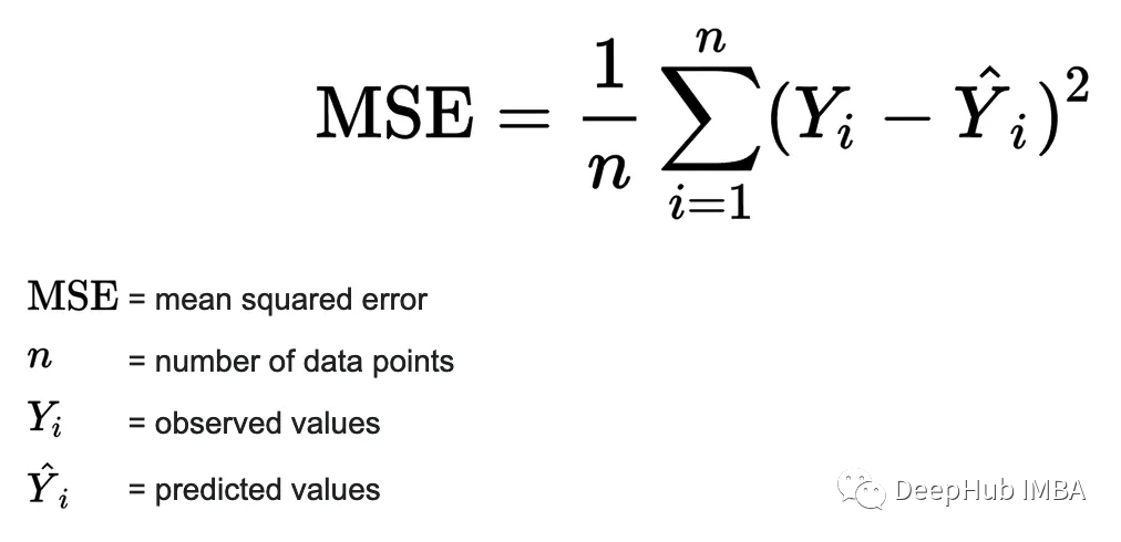
After defining the model, we can choose a loss function and optimizer, set the learning rate and number of epochs, and start our training loop. Since this is a regression problem (i.e., we are trying to predict a continuous value), the simplest and safest loss function is mean squared error. This provides a robust way to compute the error between the actual values and the model’s predictions.

The optimizer and loss function are as follows:
 # Set learning rate and number of epochs to train over
 lr = 4e-4
 n_epochs = 20
 # Initialize the loss function and optimizer
 criterion = nn.MSELoss().to(device)
 optimizer = torch.optim.AdamW(model.parameters(), lr=lr)
Below is the code for the training loop: In each training iteration, we will compute the loss for the training and validation sets that we created earlier:
# Lists to store training and validation losses
t_losses, v_losses = [], []
# Loop over epochs
for epoch in range(n_epochs):
    train_loss, valid_loss = 0.0, 0.0
    # train step
    model.train()
    # Loop over train dataset
    for x, y in trainloader:
        optimizer.zero_grad()
        # move inputs to device
        x = x.to(device)
        y  = y.squeeze().to(device)
        # Forward Pass
        preds = model(x).squeeze()
        loss = criterion(preds, y)  # compute batch loss
        train_loss += loss.item()
        loss.backward()
        optimizer.step()
    epoch_loss = train_loss / len(trainloader)
    t_losses.append(epoch_loss)
    # validation step
    model.eval()
    # Loop over validation dataset
    for x, y in testloader:
        with torch.no_grad():
            x, y = x.to(device), y.squeeze().to(device)
            preds = model(x).squeeze()
            error = criterion(preds, y)
        valid_loss += error.item()
    valid_loss = valid_loss / len(testloader)
    v_losses.append(valid_loss)
    print(f'{epoch} - train: {epoch_loss}, valid: {valid_loss}')
plot_losses(t_losses, v_losses)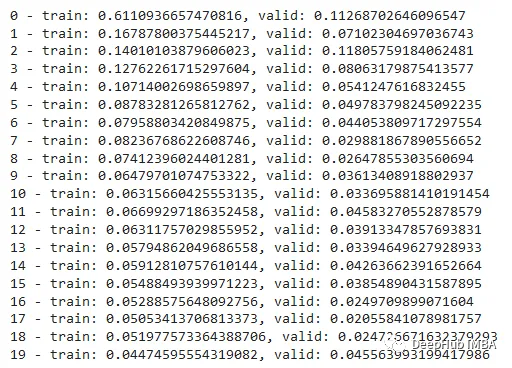
Now the model is trained and can be evaluated for predictions.
Inference
We call the trained model to predict on the unshuffled data and compare how different the predictions are from the actual observations.
def make_predictions_from_dataloader(model, unshuffled_dataloader):
    model.eval()
    predictions, actuals = [], []
    for x, y in unshuffled_dataloader:
        with torch.no_grad():
            p = model(x)
            predictions.append(p)
            actuals.append(y.squeeze())
    predictions = torch.cat(predictions).numpy()
    actuals = torch.cat(actuals).numpy()
    return predictions.squeeze(), actuals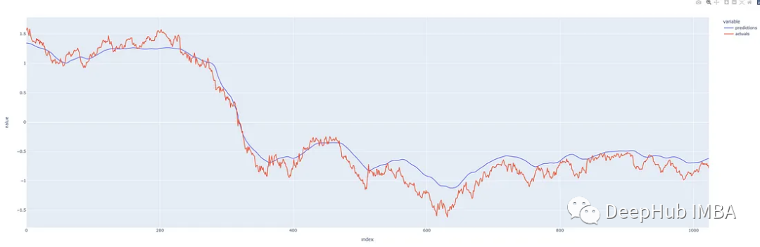
Our predictions look quite good! The prediction performance is decent, indicating that we have not overfitted the model. Let’s see if we can use it to predict the future.
Prediction
If we define history as the sequence before the moment of prediction, the algorithm is simple:
-
Obtain the latest valid sequence from history (length of training window).
-
Input the latest sequence into the model and predict the next value.
-
Append the predicted value to the history.
-
Iterate and repeat step 1.
Here, it’s important to note that the longer you predict (further) based on the parameters chosen when training the model, the more the model may exhibit its own bias, starting to predict the average value. Therefore, unless necessary, we do not want to always predict too far ahead, as this can affect the accuracy of the prediction.
This is implemented in the function below:
def one_step_forecast(model, history):
    '''
    model: PyTorch model object
    history: a sequence of values representing the latest values of the time series, requirement -> len(history.shape) == 2
    outputs a single value which is the prediction of the next value in the sequence.
    '''
    model.cpu()
    model.eval()
    with torch.no_grad():
        pre = torch.Tensor(history).unsqueeze(0)
        pred = self.model(pre)
    return pred.detach().numpy().reshape(-1)

def n_step_forecast(data: pd.DataFrame, target: str, tw: int, n: int, forecast_from: int=None, plot=False):
    '''
    n: integer defining how many steps to forecast
    forecast_from: integer defining which index to forecast from. None if you want to forecast from the end.
    plot: True if you want to output a plot of the forecast, False if not.
    '''
    history = data[target].copy().to_frame()
    # Create initial sequence input based on where in the series to forecast
    # from.
    if forecast_from:
        pre = list(history[forecast_from - tw : forecast_from][target].values)
    else:
        pre = list(history[self.target])[-tw:]
    # Call one_step_forecast n times and append prediction to history
    for i, step in enumerate(range(n)):
        pre_ = np.array(pre[-tw:]).reshape(-1, 1)
        forecast = self.one_step_forecast(pre_).squeeze()
        pre.append(forecast)
    # The rest of this is just to add the forecast to the correct time of
    # the history series
    res = history.copy()
    ls = [np.nan for i in range(len(history))]
    # Note: I have not handled the edge case where the start index + n is
    # before the end of the dataset and crosses past it.
    if forecast_from:
        ls[forecast_from : forecast_from + n] = list(np.array(pre[-n:]))
        res['forecast'] = ls
        res.columns = ['actual', 'forecast']
    else:
        fc = ls + list(np.array(pre[-n:]))
        ls = ls + [np.nan for i in range(len(pre[-n:]))]
        ls[:len(history)] = history[self.target].values
        res = pd.DataFrame([ls, fc], index=['actual', 'forecast']).T
    return res
Let’s take a look at the actual effects.
We make predictions from different points in the middle of this time series so that we can compare the predictions with what actually happened. Our prediction program can predict from anywhere for any reasonable number of steps, with the red line indicating the forecast. (These charts show standardized prices on the y-axis)
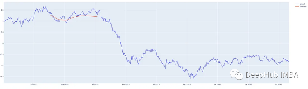
Prediction 200 days after Q3 2013
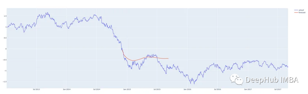
Prediction 200 days after 2014/15
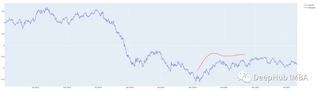
Prediction 200 days from the first quarter of 2016
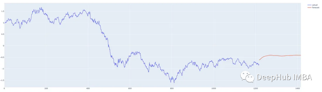
Prediction 200 days from the last day of the data
Summary
Our model performs fairly well! However, we have presented the entire process of time series prediction through this example. We can improve the model and make more accurate predictions by trying different architectures and tuning parameters.
This article only deals with univariate time series, where there is only one value sequence. There are also methods to use multiple series for predictions. This is called multivariate time series forecasting, which I will cover in future articles.