New Intelligence Column
Author: Zhang Hao (Nanjing University)
This article is sourced from: New Intelligence
【Introduction】Deep learning has become one of the fastest growing and most exciting fields in machine learning. This article introduces key concepts in computer vision, highlighting the applications of deep learning in tasks such as network compression, fine-grained image classification, image captioning, visual question answering, image understanding, texture generation, style transfer, face recognition, image retrieval, and object tracking.

Despite the excellent performance of deep neural networks, the enormous computational and storage costs pose challenges for their deployment in practical applications. Research shows that there is a significant amount of redundancy in the parameters of neural networks. Therefore, many efforts are focused on reducing network complexity while maintaining accuracy.
Low-Rank Approximation is used to approximate the original weight matrix with a low-rank matrix. For example, the optimal low-rank approximation of the original matrix can be obtained using SVD, or the original matrix can be approximated using a Toeplitz matrix combined with Krylov decomposition.
Pruning (pruning) After training, some unimportant neuron connections (which can be measured by the size of weight values in conjunction with sparsity constraints in the loss function) or entire filters can be removed, followed by several rounds of fine-tuning. In practice, pruning at the neuron connection level can make the results sparse, which is not conducive to cache optimization and memory access, and some may require specially designed accompanying runtime libraries. In contrast, filter-level pruning can run directly on existing runtime libraries, and the key to filter-level pruning is how to measure the importance of filters. For example, the sparsity of convolution results, the impact of that filter on the loss function, or the influence of convolution results on the next layer’s results can be used for measurement.
Quantization (quantization) clusters weight values, replacing the original weight values with the cluster centers, combined with Huffman coding, which may include scalar quantization or product quantization. However, if only the weights themselves are considered, it can easily lead to a situation where quantization error is low but classification error is high. Therefore, the optimization goal of Quantized CNN is to minimize reconstruction error. Additionally, hashing can be used for encoding, meaning that weights mapped to the same hash bucket share the same parameter value.
Reducing the Range of Data Values By default, data is represented as single-precision floating-point numbers, occupying 32 bits. Research has found that switching to half-precision floating-point numbers (16 bits) has little effect on performance. Google’s TPU uses 8-bit integers to represent data. In extreme cases, the value range can be binary or ternary (0/1 or -1/0/1), allowing all computations to be completed quickly using bit operations; however, how to train binary or ternary networks is key. The usual approach is that the feedforward process of the network is binary or ternary, while the gradient update process uses real values. Additionally, some research suggests that the representational capacity of binary operations is limited, hence an additional floating-point number is used to scale the results of binary convolutions to enhance the network’s representational capability.
Simplified Structural Design Some research directly designs simplified network structures. For example, (1). Bottleneck structure and 1×1 convolution. This design philosophy has been widely used in the Inception and ResNet series of network designs. (2). Grouped Convolution. (3). Dilated Convolution. Using dilated convolution can expand the receptive field while keeping the parameter count unchanged.
Knowledge Distillation (knowledge distillation) trains a small network to approximate a large network, but how to approach the large network is still inconclusive.
Co-design of Software and Hardware Commonly used hardware includes two main categories: (1). General-purpose hardware, including CPU (low latency, good at serial and complex computations) and GPU (high throughput, good at parallel and simple computations). (2). Specialized hardware, including ASIC (fixed logic devices, e.g., Google TPU) and FPGA (programmable logic devices, flexible but less efficient than ASIC).
Compared with (general) image classification, fine-grained image classification requires more precise judgment of the image categories. For example, we need to determine which specific bird, which model of car, or which type of airplane the target is. Typically, the differences between these subclasses are very subtle. For instance, the visible difference between Boeing 737-300 and Boeing 737-400 is only the number of windows.
Classic approaches to fine-grained image classification first locate different parts of the target, such as the head, feet, and wings of a bird, and then extract features for these parts separately, finally merging these features for classification. These methods have higher accuracy, but they require manual labeling of part information in the dataset. Currently, a major research trend in fine-grained classification is to learn using only image labels without additional supervisory information, represented by methods based on bilinear CNN.
Bilinear CNN (bilinear CNN) examines the interaction between different dimensions by calculating the outer product of convolution descriptor vectors. Since different dimensions of the descriptor vector correspond to different channels of convolution features, and different channels extract different semantic features, bilinear operations can capture the relationships between different semantic features of the input image simultaneously.
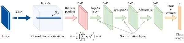
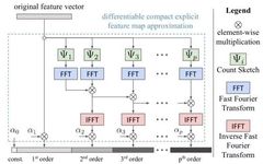
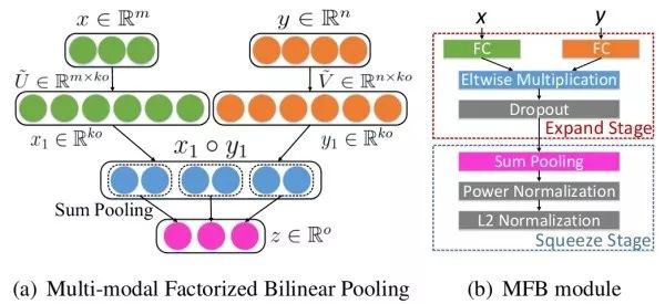
Simplified Bilinear Pooling The results of bilinear pooling are high-dimensional, which consumes a lot of computational and storage resources, and significantly increases the parameter count of subsequent fully connected layers. Many subsequent research works aim to design more streamlined bilinear pooling strategies, roughly including the following three categories: (1). PCA dimensionality reduction. Before bilinear pooling, project the deep descriptor vector using PCA for dimensionality reduction, but this can make the dimensions no longer correlated, thereby affecting performance. A compromise is to only perform PCA dimensionality reduction on one branch. (2). Approximate Kernel Estimation. It can be proven that using linear SVM classification after bilinear pooling results is equivalent to using a polynomial kernel between descriptor vectors. Since the mapping of the outer product of two vectors is equal to convolving the two vectors after mapping them separately, some research uses random matrices to approximate the mapping of vectors. Additionally, through approximate kernel estimation, we can capture information beyond the second order (as shown below). (3). Low-Rank Approximation. Perform low-rank approximation on the parameter matrix of the fully connected layer used for classification, thereby eliminating the need to explicitly compute the results of bilinear pooling.

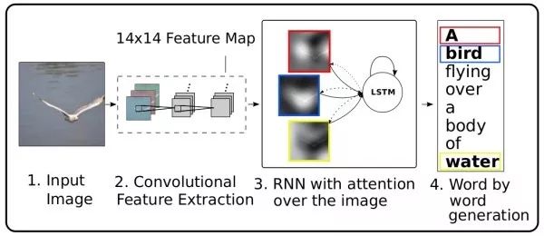
Image captioning aims to generate a one or two-sentence textual description of an image’s content. This is a cross-task between the fields of vision and natural language processing.
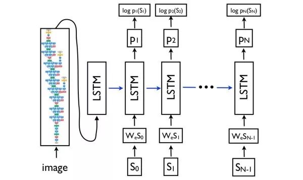
Encoder-Decoder Networks The basic idea behind image captioning network design is inspired by machine translation in natural language processing. The source language encoding network in machine translation is replaced by a CNN encoding network for images to extract image features, and then a target language decoding network generates textual descriptions.
Show, Attend, and Tell The attention mechanism is a common technique used in machine translation to capture long-distance dependencies, and it can also be used in image captioning. In the decoding network, at each moment, in addition to predicting the next word, a two-dimensional attention map needs to be output to weight the deep convolution features. An additional benefit of using the attention mechanism is that it allows for visualization of the network to observe which parts of the image the network focuses on when generating each word.
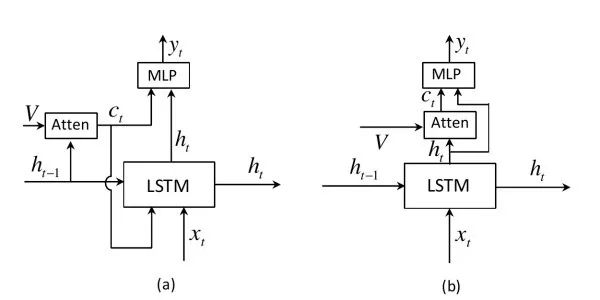
Adaptive Attention The previous attention mechanism generates a two-dimensional attention map for each word to be predicted (Fig. (a)), but for words like “the” and “of,” there is no need for image clues, and some words can also be inferred from context. This work extends LSTM to propose a “visual sentinel” mechanism to determine whether to focus more on contextual language information or image information when predicting the current word (Fig. (b)). Additionally, unlike previous works that use the previous hidden state to calculate the attention map, this work uses the current hidden state.
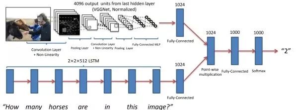
Given an image and a text question about the content of that image, visual question answering aims to select the correct answer from several candidate text responses. Essentially, it is a classification task, and some works also use RNN decoding to generate text answers. Visual question answering is also a cross-task between the fields of vision and natural language processing.
Basic Idea Use CNN to extract image features from the image, use RNN to extract text features from the text question, and then attempt to fuse visual and textual features, finally classifying through a fully connected layer. The key to this task is how to fuse these two modalities’ features. A direct fusion scheme is to concatenate the visual and textual features into a vector or to add or multiply the visual and textual feature vectors element-wise.
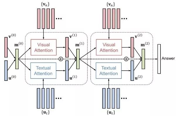
Attention Mechanism Similar to image captioning, using the attention mechanism can also improve the performance of visual question answering. The attention mechanism includes visual attention (“where to look”) and textual attention (“which word to focus on”). HieCoAtten can generate visual and textual attention simultaneously or alternately. DAN maps the results of visual and textual attention to the same space and produces the next visual and textual attention based on that.
Bilinear Fusion By taking the outer product of the visual feature vector and the textual feature vector, the interaction between the dimensions of these two modalities’ features can be captured. To avoid explicitly calculating the high-dimensional bilinear pooling results, the idea of simplified bilinear pooling in fine-grained recognition can also be applied to visual question answering. For example, MFB adopts the low-rank approximation idea and simultaneously uses the visual and textual attention mechanisms.
These methods aim to provide some visualization tools to understand deep convolutional neural networks.
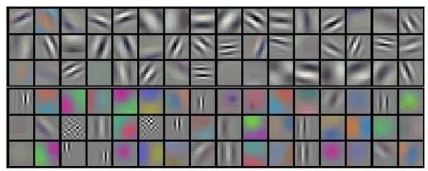
Direct Visualization of the First Layer Filters Since the filters of the first convolutional layer slide directly over the input image, we can visualize the first layer filters directly. It can be seen that the first layer weights focus on edges of specific orientations and certain color combinations. This aligns with biological visual mechanisms. However, since high-level filters do not directly act on the input image, direct visualization is only effective for the first layer filters.
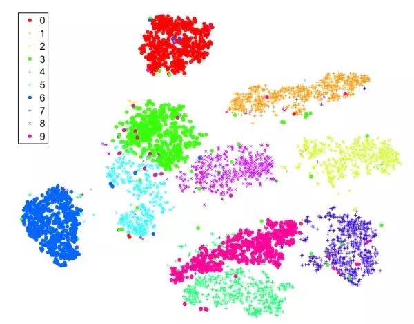
t-SNE Low-dimensional embeddings of features from fc7 or pool5 of images, for example, reducing dimensions to 2D to visualize them on a two-dimensional plane. Images with similar semantic information should be close together in the t-SNE results. Unlike PCA, t-SNE is a nonlinear dimensionality reduction method that preserves local distances. The following image shows the t-SNE results directly applied to the original MNIST images. It can be seen that MNIST is a relatively easy dataset, with clear clustering of images belonging to different categories.
Visualizing Intermediate Layer Activation Values For a given input image, plot the responses of different feature maps. It is observed that even if there are no face or text-related categories in ImageNet, the network learns to recognize these semantic features to assist in subsequent classification.
Max Response Regions of Images Select a specific intermediate layer neuron, input many different images into the network, and find the image regions that produce the maximum response for that neuron to observe which semantic features that neuron responds to. It is the “image region” rather than the “entire image” because the receptive field of intermediate layer neurons is limited and does not cover the entire image.
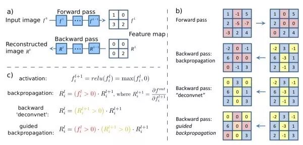
Input Saliency Maps For a given input image, calculate the partial derivative of a specific neuron with respect to the input image. This expresses the influence of different pixels of the input image on the response of that neuron, i.e., how changes in different pixels of the input image will affect the changes in the neuron’s response value. Guided backprop only backpropagates positive gradient values, focusing only on the positive influence on the neuron, which produces better visualization results than standard backpropagation.
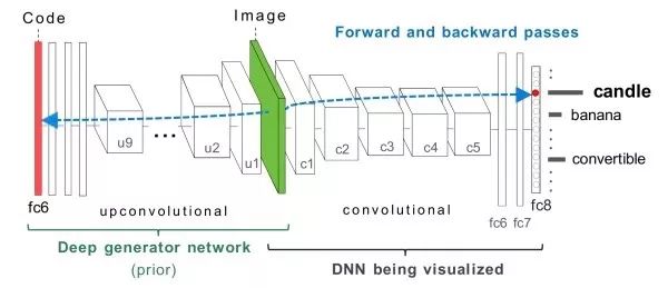
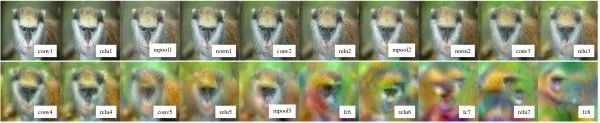
Gradient Ascent Optimization Select a specific neuron, calculate the partial derivative of that neuron with respect to the input image, and optimize the input image using gradient ascent until convergence. Additionally, we need some regularization terms to make the generated image closer to a natural image. Furthermore, instead of optimizing the input image, we can also optimize the fc6 features and generate the desired image from them.
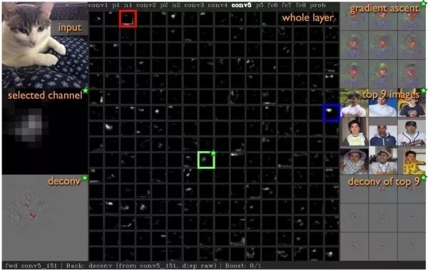
DeepVisToolbox This toolbox provides the above four visualization results simultaneously. A demonstration video is available at this link: Jason Yosinski (yosinski.com/deepvis#toolbox)
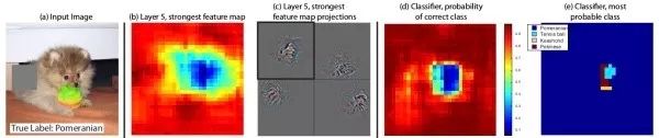
Occlusion Experiment (occlusion experiment) Use a gray square to occlude different regions of the image, then feed it through the network to observe its impact on the output. The region that has the greatest impact on the output is the most important region for determining that category. From the following image, it can be seen that occluding the dog’s face has the greatest impact on the result.
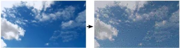
Deep Dream Select an image and a specific layer, optimizing the goal is to maximize the square of the activation value of that layer through gradient ascent on the image. In practice, this amplifies the semantic features captured by that layer’s neurons through positive feedback. It can be observed that many dog patterns appear in the generated image because there are 200 classes related to dogs in the ImageNet dataset, so many neurons in the neural network are dedicated to recognizing dogs in images.
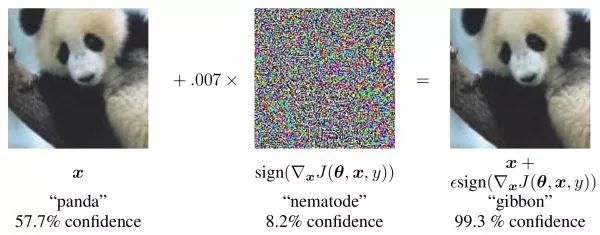
Adversarial Examples (adversarial examples) Select an image and a category that is not its true label, calculate the partial derivative of that category with respect to the input image, and perform gradient ascent optimization on the image. Experiments have shown that after making imperceptible small changes to the image, the network can be made to confidently classify the image as belonging to the wrong category. In practical applications, adversarial examples pose threats in fields such as finance and security. Some research suggests that this is due to the high dimensionality of the image space, where even with a large amount of training data, only a small part of the space can be covered. As long as the input slightly deviates from that manifold space, the network struggles to make normal judgments.
Given a small image containing a specific texture, texture synthesis aims to generate a larger image containing the same texture. Given a normal image and an image containing a specific painting style, style transfer aims to retain the content of the original image while transferring the given style to that image.
Feature Inversion (feature inversion) This is the basic idea for both problems. Given an intermediate layer feature, we aim to generate an image that closely resembles the given feature through iterative optimization. Additionally, feature inversion can tell us how much information is contained in the image from the intermediate layer features. It can be observed that low-level features contain almost no loss of image information, while high-level features, especially fully connected features, tend to lose most of the detailed information. On the other hand, high-level features are less sensitive to changes in color and texture of the image.
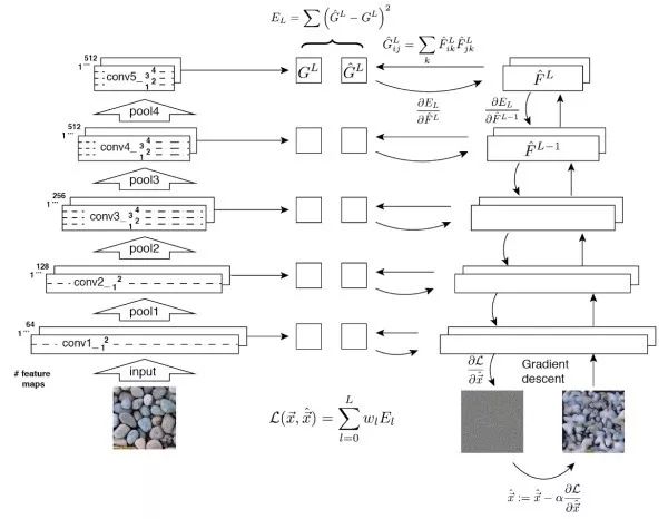
Gram Matrix GivenD×H×W depth convolution features, we convert it to aD×(HW) matrixX, then the Gram matrix corresponding to that layer’s features is defined as
G=XX^T
Through the outer product, the Gram matrix captures the co-occurrence relationships between different features.
Basic Idea of Texture Generation Perform feature inversion on the Gram matrix of the given texture pattern. Make the Gram matrices of the layers of the generated image’s features close to those of the given texture image. Low-level features tend to capture detailed information, while high-level features can capture larger area features.
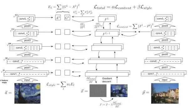
Basic Idea of Style Transfer The optimization objectives include two parts: to make the content of the generated image close to that of the original image, and to make the style of the generated image close to the given style. The style is represented by the Gram matrix, while the content is directly represented by the neuron activation values.
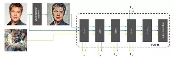
Directly Generating Style Transfer Images The disadvantage of the above method is that it requires multiple iterations to converge. The solution proposed by this work is to train a neural network to directly generate style transfer images. Once the training is complete, performing style transfer only requires a single feedforward through the network, making it very efficient. During training, the generated image, original image, and style image are fed through a fixed network to extract different layer features for loss function calculation.
Instance Normalization (instance normalization) and batch normalization operate differently on a batch. The mean and variance of instance normalization are determined solely by the image itself. Experiments have shown that using instance normalization in style transfer networks can remove contrast information related to the instance from the image to simplify the generation process.
Conditional Instance Normalization (conditional instance normalization) A problem with the above method is that for each different style, we need to train a separate model. Due to the commonalities between different styles, this work aims to allow the style transfer networks corresponding to different styles to share parameters. Specifically, it modifies the instance normalization in the style transfer network to have N sets of scaling and shifting parameters, each corresponding to a different style. This way, we can obtain N style transfer images simultaneously through a single feedforward process.
Face verification/recognition can be considered a more refined fine-grained image recognition task. Face verification determines whether two images belong to the same person, while face recognition identifies who the person in the image is. A face verification/recognition system typically includes three main steps: detecting faces in images, locating feature points, and verifying/recognizing the faces. The challenge of face verification/recognition lies in the need for few-shot learning. Typically, there is only one corresponding image per person in the dataset, known as one-shot learning.
Two Basic Approaches Treat it as a classification problem (facing a very large number of categories), or treat it as a metric learning problem. If two images belong to the same person, we hope their deep features are close; otherwise, we hope they are not close. Then, based on the distance between the deep features, we perform verification (setting a threshold for feature distance to determine whether they belong to the same person) or recognition (k-nearest neighbor classification).
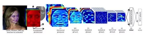
DeepFace The first model to successfully apply deep neural networks to face verification/recognition. DeepFace uses non-shared parameters in local connections. This is because different regions of the face have different features (e.g., eyes and mouth have different features), and the “shared parameters” nature of classic convolutional layers is not suitable for face recognition. Therefore, face recognition networks adopt local connections without shared parameters. It uses a Siamese network for face verification. When the deep features of two images are less than a given threshold, they are considered to come from the same person.
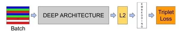
FaceNet uses a triplet input, hoping that the distance between the negative sample and the positive sample is greater than a certain margin (e.g., 0.2). Additionally, the selection of input triplets is not random; otherwise, due to the large differences with the negative samples, the network cannot learn effectively. Selecting the hardest triplets (i.e., the farthest positive sample and the nearest negative sample) can lead the network to get stuck in local optima. FaceNet adopts a semi-hard strategy, selecting negative samples that are farther than the positive samples.

Large Margin Cross-Entropy Loss In recent years, a major research focus has been on this topic. Due to large intra-class variability and high inter-class similarity, some research aims to enhance the judgment capability of classic cross-entropy loss on deep features. For example, L-Softmax strengthens the optimization goal, increasing the angle between the parameter vector corresponding to the class and the deep feature. A-Softmax further constrains the length of the parameter vector of L-Softmax to 1, making training more focused on optimizing deep features and angles. In practice, both L-Softmax and A-Softmax are difficult to converge, so an annealing method is used during training, gradually transitioning from standard softmax to L-Softmax or A-Softmax.
Liveness Detection (liveness detection) determines whether the face comes from a real person or a photo, which is a key issue that needs to be addressed in face verification/recognition. The mainstream approach in the industry currently involves using changes in facial expressions, texture information, blinking, or having users perform a series of actions.
Given a query image containing a specific instance (such as a specific object, scene, or building), image retrieval aims to find images in a database that contain the same instance. However, due to different shooting angles, lighting, or occlusion conditions of different images, designing effective and efficient image retrieval algorithms that can cope with these intra-class differences remains a research challenge.
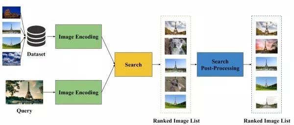
Typical Process of Image Retrieval First, attempt to extract a suitable representation vector from the image. Second, perform nearest neighbor search using Euclidean distance or cosine distance on these representation vectors to find similar images. Finally, some post-processing techniques can be used to fine-tune the retrieval results. It can be seen that the key to determining the performance of an image retrieval algorithm is the quality of the extracted image representation.
(1) Unsupervised Image Retrieval
Unsupervised image retrieval aims to utilize a fixed feature extractor, such as the ImageNet pre-trained model, to extract image representations without relying on other supervisory information.
Intuitive Idea Since deep fully connected features provide high-level descriptions of image content and are in a “natural” vector form, an intuitive idea is to directly extract deep fully connected features as the image representation vector. However, since fully connected features are designed for image classification and lack detailed descriptions of the image, the retrieval accuracy of this approach is generally low.
Using Deep Convolution Features Since deep convolution features have better detail information and can handle images of arbitrary sizes, the current mainstream method is to extract deep convolution features and obtain the image representation vector through weighted global sum pooling. The weights reflect the importance of features at different positions, which can take two forms: spatial direction weights and channel direction weights.
CroW Deep convolution features are a distributed representation. Although the response value of a single neuron is not very useful for determining whether the corresponding region contains the target, if multiple neurons have large response values simultaneously, that region is likely to contain the target. Therefore, CroW sums the feature maps along the channel direction to obtain a two-dimensional aggregation map, normalizes it, and uses the square root normalized result as the spatial weight. The channel weights of CroW are defined based on the sparsity of the feature maps, similar to the IDF feature in TF-IDF in natural language processing, which is used to enhance the discriminative capability of infrequently occurring features.
Class Weighted Features This method attempts to combine the category prediction information of the network to make the spatial weights more discriminative. Specifically, it uses CAM to obtain semantic information from the most representative regions corresponding to each category in the pre-trained network, and then normalizes the CAM results as spatial weights.
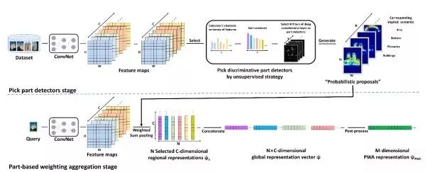
PWA PWA finds that different channels of deep convolution features correspond to responses from different parts of the target. Therefore, PWA selects a series of discriminative feature maps, normalizes the results, and uses them as spatial weights for pooling, concatenating the results as the final image representation.
(2) Supervised Image Retrieval
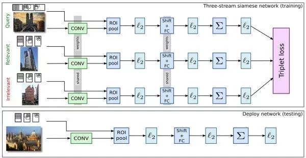
Supervised image retrieval first fine-tunes the ImageNet pre-trained model on an additional training dataset, and then extracts image representations from this fine-tuned model. To achieve better results, the training dataset used for fine-tuning is usually quite similar to the dataset to be used for retrieval. Additionally, candidate region networks can be used to extract the foreground regions of the images that may contain the target.
Siamese Network (siamese network) Similar to the idea of face recognition, it uses binary or triplet (++-) inputs to train the model to minimize the distance between similar samples while maximizing the distance between dissimilar samples.
Object tracking aims to track the movement of a target in a video. Typically, the position of the target in the first frame of the video is given in the form of a bounding box, and we need to predict the bounding box of that target in subsequent frames. Object tracking is similar to object detection, but the difficulty of object tracking lies in the fact that the specific target to be tracked is not known in advance, making it impossible to collect enough training data to train a dedicated detector.
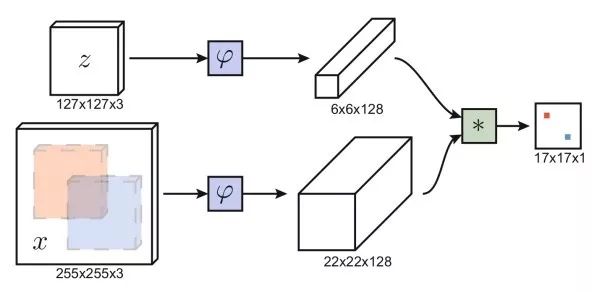
Siamese Network Similar to the idea of face verification, using a Siamese network, one branch inputs the image within the bounding box of the first frame, while the other branch inputs candidate image regions from other frames, outputting the similarity between the two images. We do not need to traverse all possible candidate regions in other frames; using a fully convolutional network, we only need to feed the entire image once. By performing cross-correlation operations (convolution), we obtain a two-dimensional response map, where the position of the maximum response determines the predicted bounding box location. The Siamese network-based method is fast and can handle images of any size.
CFNet Correlation filtering distinguishes image regions from their surrounding areas by training a linear template, and through Fourier transform, correlation filtering has very efficient implementations. CFNet combines the offline-trained Siamese network with an online-updated correlation filtering module to enhance the tracking performance of lightweight networks.

These models aim to learn the distribution of data (images) or sample new images from that distribution. Generative models can be used for super-resolution reconstruction, image coloring, image transformation, generating images from text, learning latent representations of images, semi-supervised learning, and more. Additionally, generative models can be combined with reinforcement learning for simulation and inverse reinforcement learning.
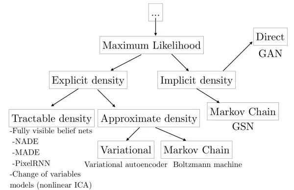
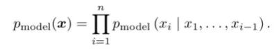
Explicit Modeling Directly learning the distribution of images through maximum likelihood estimation according to the conditional probability formula. The drawback of this method is that since each pixel depends on the previous pixels, generating images needs to be done sequentially starting from one corner, which can be quite slow. For example, WaveNet can generate speech similar to human speech, but due to the inability to generate in parallel, generating 1 second of speech requires 2 minutes of computation, making it impractical for real-time applications.
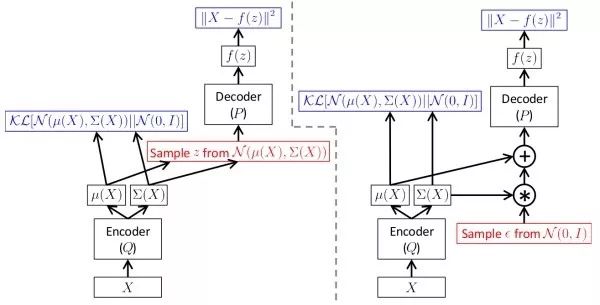
Variational Auto-Encoder (variational auto-encoder, VAE) To avoid the drawbacks of explicit modeling, variational auto-encoders perform implicit modeling of data distributions. They assume that the generation of images is controlled by a latent variable, which is assumed to follow a diagonal Gaussian distribution. Variational auto-encoders generate images from latent variables through a decoding network. Since direct maximum likelihood estimation cannot be performed, during training, similar to the EM algorithm, variational auto-encoders construct a lower bound function for the likelihood function and optimize this lower bound function. The advantage of variational auto-encoders is that, due to the independence of each dimension, we can control the factors of variation in the output images by manipulating the latent variables.
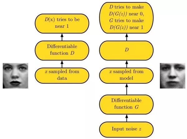
Generative Adversarial Networks (generative adversarial networks, GAN) Due to the difficulty of learning data distributions, generative adversarial networks bypass this step and generate new images directly. Generative adversarial networks use a generator network G to generate images from random noise, and a discriminator network D to determine whether the input images are real or fake. During training, the goal of the discriminator network D is to judge real/fake images, while the goal of the generator network G is to make the discriminator network D inclined to judge its output as a real image. In practice, directly training generative adversarial networks encounters the mode collapse problem, where the generative adversarial network fails to learn the complete data distribution. Subsequently, improvements like LS-GAN and W-GAN emerged. Compared to variational auto-encoders, generative adversarial networks provide better detail information. The following link organizes many papers related to generative adversarial networks: hindupuravinash/the-gan-zoo. The following link organizes various techniques for training generative adversarial networks: soumith/ganhacks.
Most of the tasks introduced earlier can also be applied to video data; here we take video classification as an example to briefly introduce the basic methods for processing video data.
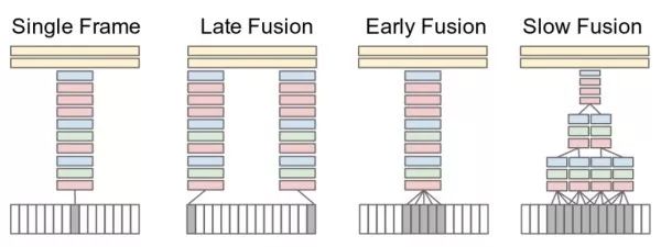
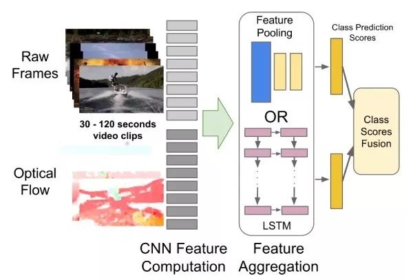
Multi-Frame Image Feature Pooling These methods treat videos as a combination of a series of frames. The network simultaneously receives several frames of images belonging to a video segment (e.g., 15 frames), extracts their deep features separately, and then merges these image features to obtain the features of that video segment, followed by classification. Experiments have found that using “slow fusion” yields the best results. Additionally, independently using single-frame images for classification can yield competitive results, indicating that single-frame images contain a lot of information.
3D Convolution Extending classic 2D convolution to 3D convolution, allowing local connections in the temporal dimension as well. For example, the 3×3 convolution of VGG can be extended to a 3×3×3 convolution, and the 2×2 pooling can be extended to a 2×2×2 pooling.
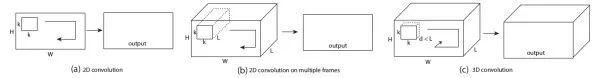
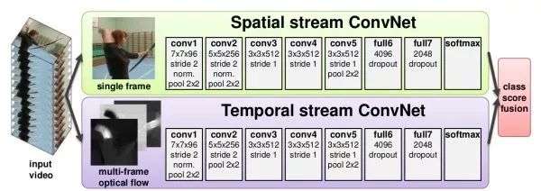
Image + Temporal Two-Branch Structure These methods use two independent networks to capture image information and motion information over time in the video. The image information is obtained from single-frame still images, which is a classic image classification problem. The motion information is captured through optical flow, which captures the motion of the target between adjacent frames.
CNN + RNN Capturing Long-Distance Dependencies Previous methods could only capture dependencies between a few frames of images, while this method aims to use CNN to extract features from single-frame images and then use RNN to capture dependencies between frames.
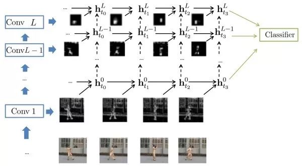
In addition, some research works attempt to combine CNN and RNN into one, allowing each convolutional layer to capture long-distance dependencies.
Author Introduction
Zhang Hao: A master’s student at the School of Computer Science, Nanjing University, specializing in machine learning and data mining (LAMDA), with research interests in computer vision and machine learning, especially visual recognition and deep learning. Personal homepage: http://lamda.nju.edu.cn/zhangh/.
📚 Previous Articles Recommended

Submission Email: [email protected]
Long press the QR code below to subscribe for free!
How to Join the Society
Register as a Society Member:
Individual Membership:
Follow the WeChat of the Society: China Command and Control Society (c2_china), reply “individual member” to obtain the membership application form, fill it out as required, and if there are any questions, you can message within the public account. Only after passing the society’s review can you pay the membership fee online via Alipay.
Institutional Membership:
Follow the WeChat of the Society: China Command and Control Society (c2_china), reply “institutional member” to obtain the membership application form, fill it out as required, if there are any questions, you can message within the public account. Only after passing the society’s review can you pay the membership fee.
Long press the QR code below to follow the society’s WeChat

Thank you for your attention