
About 5200 words, recommended reading time 10 minutes.
This article summarizes commonly used deep learning models, providing an in-depth introduction to their principles and applications.
-
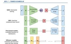
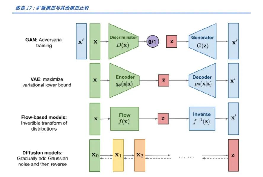
Encoder: Encodes the input data x into the mean μ and standard deviation σ of the latent variable z. -
Sampling: Samples an ε from the standard normal distribution, calculates z = μ + ε * σ. -
Decoder: Decodes z into generated samples x’. -
Calculates reconstruction error (such as MSE) and KL divergence, optimizing model parameters to minimize their sum.
-
Can generate diverse samples. -
The latent variables have a clear probabilistic interpretation.
-
The training process can be unstable. -
The quality of generated samples may not be as good as other models.
-
Data generation and interpolation. -
Feature extraction and dimensionality reduction.
import torch
import torch.nn as nn
import torch.optim as optim
class VAE(nn.Module):
    def __init__(self, input_dim, hidden_dim):
        super(VAE, self).__init__()
        self.encoder = nn.Sequential(
            nn.Linear(input_dim, hidden_dim),
            nn.ReLU(),
            nn.Linear(hidden_dim, 2 * hidden_dim)  # Mean and standard deviation
        )
        self.decoder = nn.Sequential(
            nn.Linear(hidden_dim, hidden_dim),
            nn.ReLU(),
            nn.Linear(hidden_dim, input_dim),
            nn.Sigmoid()  # Binary data, use Sigmoid activation function
        )
    def reparameterize(self, mu, logvar):
        std = torch.exp(0.5 * logvar)
        eps = torch.randn_like(std)
        return mu + eps * std
    def forward(self, x):
        h = self.encoder(x)
        mu, logvar = h.chunk(2, dim=-1)
        z = self.reparameterize(mu, logvar)
        x_recon = self.decoder(z)
        return x_recon, mu, logvar
# Example training process
model = VAE(input_dim=784, hidden_dim=400)
optimizer = optim.Adam(model.parameters(), lr=1e-3)
# Assume x is input data, batch_size is batch size
x = torch.randn(batch_size, 784)
recon_x, mu, logvar = model(x)
loss = nn.functional.binary_cross_entropy(recon_x, x, reduction='sum') + 0.5 * torch.sum(torch.exp(logvar) + mu.pow(2) - 1 - logvar)
optimizer.zero_grad()
loss.backward()
optimizer.step()
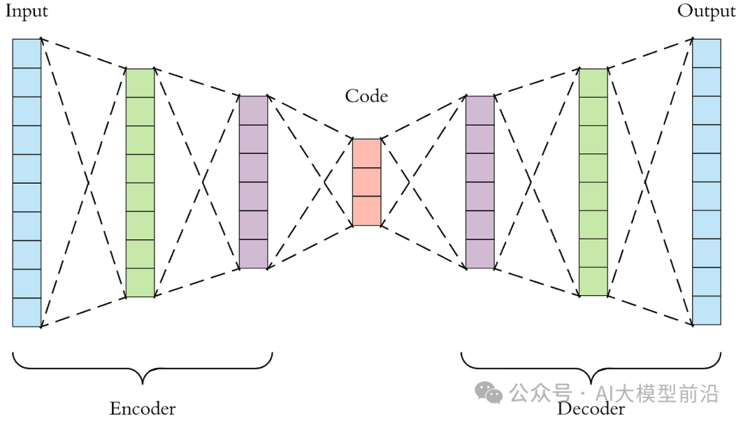
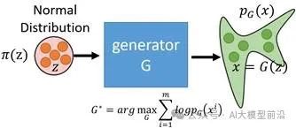
-
The discriminator receives real data and fake data generated by the generator, training in a binary classification manner to optimize its ability to judge real or generated data. -
The generator attempts to generate more realistic fake data to deceive the discriminator based on the feedback from the discriminator. -
Alternately train the discriminator and generator until the discriminator can no longer distinguish between real and generated data or reaches a preset number of training rounds.
-
Can generate high-quality samples. -
The training process is relatively free and not limited by data distribution.
-
Training can be unstable and easily fall into local optima. -
Requires a large amount of computational resources.
-
Image generation. -
Text generation. -
Speech recognition, etc.
import torch
import torch.nn as nn
import torch.optim as optim
# Discriminator
class Discriminator(nn.Module):
    def __init__(self, input_dim):
        super(Discriminator, self).__init__()
        self.fc = nn.Sequential(
            nn.Linear(input_dim, 128),
            nn.LeakyReLU(0.2),
            nn.Linear(128, 1),
            nn.Sigmoid()
        )
    def forward(self, x):
        return self.fc(x)
# Generator
class Generator(nn.Module):
    def __init__(self, input_dim, output_dim):
        super(Generator, self).__init__()
        self.fc = nn.Sequential(
            nn.Linear(input_dim, 128),
            nn.ReLU(),
            nn.Linear(128, output_dim),
            nn.Tanh()
        )
    def forward(self, x):
        return self.fc(x)
# Example training process
discriminator = Discriminator(input_dim=784)
generator = Generator(input_dim=100, output_dim=784)
optimizer_D = optim.Adam(discriminator.parameters(), lr=0.0002)
optimizer_G = optim.Adam(generator.parameters(), lr=0.0002)
criterion = nn.BCEWithLogitsLoss()
# Assume real_data is real data, batch_size is batch size
real_data = torch.randn(batch_size, 784)
# Train the discriminator
for p in discriminator.parameters():
    p.requires_grad = True
for p in generator.parameters():
    p.requires_grad = False
noise = torch.randn(batch_size, 100)
fake_data = generator(noise)
real_loss = criterion(discriminator(real_data), torch.ones_like(real_data))
fake_loss = criterion(discriminator(fake_data.detach()), torch.zeros_like(real_data))
discriminator_loss = real_loss + fake_loss
optimizer_D.zero_grad()
discriminator_loss.backward()
optimizer_D.step()
# Train the generator
for p in discriminator.parameters():
    p.requires_grad = False
for p in generator.parameters():
    p.requires_grad = True
noise = torch.randn(batch_size, 100)
fake_data = generator(noise)
gen_loss = criterion(discriminator(fake_data), torch.ones_like(real_data))
optimizer_G.zero_grad()
gen_loss.backward()
optimizer_G.step()
AR (Autoregressive Model)
Model Principle:
-
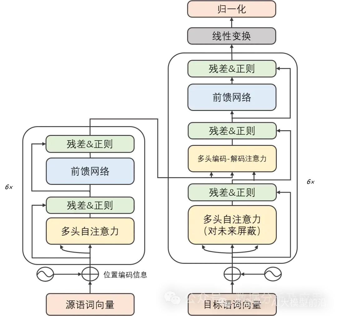
Gradient vanishing and model degradation problems are resolved: The Transformer model, with its unique self-attention mechanism, can effectively capture long-term dependencies in sequences, freeing it from the shackles of gradient vanishing and model degradation. -
Outstanding parallel computing capability: The computational architecture of the Transformer model has inherent parallelism, allowing for rapid training and inference on GPUs. -
Excellent performance across multiple tasks: With its strong feature learning and representation capabilities, the Transformer model exhibits outstanding performance in various tasks, including machine translation, text classification, and speech recognition.
-
High computational resource demand: Due to the parallelism of the Transformer model, both training and inference processes require substantial computational resource support. -
Sensitive to initialization weights: The Transformer model is highly selective about the choice of initialization weights; improper initialization can lead to training instability or overfitting issues. -
Limited handling of long-term dependencies: Although the Transformer model effectively addresses gradient vanishing and model degradation issues, it still faces challenges when processing extremely long sequences.
import torch
import torch.nn as nn
import torch.optim as optim
# This example is only for illustrating the basic structure and principles of the Transformer. Actual Transformer models (like GPT or BERT) are much more complex and require more preprocessing steps such as tokenization, padding, masking, etc.
class Transformer(nn.Module):
    def __init__(self, d_model, nhead, num_encoder_layers, num_decoder_layers, dim_feedforward=2048):
        super(Transformer, self).__init__()
        self.model_type = 'Transformer'
        # encoder layers
        self.src_mask = None
        self.pos_encoder = PositionalEncoding(d_model, max_len=5000)
        encoder_layers = nn.TransformerEncoderLayer(d_model, nhead, dim_feedforward)
        self.transformer_encoder = nn.TransformerEncoder(encoder_layers, num_encoder_layers)
        # decoder layers
        decoder_layers = nn.TransformerDecoderLayer(d_model, nhead, dim_feedforward)
        self.transformer_decoder = nn.TransformerDecoder(decoder_layers, num_decoder_layers)
        # decoder
        self.decoder = nn.Linear(d_model, d_model)
        self.init_weights()
    def init_weights(self):
        initrange = 0.1
        self.decoder.weight.data.uniform_(-initrange, initrange)
    def forward(self, src, tgt, teacher_forcing_ratio=0.5):
        batch_size = tgt.size(0)
        tgt_len = tgt.size(1)
        tgt_vocab_size = self.decoder.out_features
        # forward pass through encoder
        src = self.pos_encoder(src)
        output = self.transformer_encoder(src)
        # prepare decoder input with teacher forcing
        target_input = tgt[:, :-1].contiguous()
        target_input = target_input.view(batch_size * tgt_len, -1)
        target_input = torch.autograd.Variable(target_input)
        # forward pass through decoder
        output2 = self.transformer_decoder(target_input, output)
        output2 = output2.view(batch_size, tgt_len, -1)
        # generate predictions
        prediction = self.decoder(output2)
        prediction = prediction.view(batch_size * tgt_len, tgt_vocab_size)
        return prediction[:, -1], prediction
class PositionalEncoding(nn.Module):
    def __init__(self, d_model, max_len=5000):
        super(PositionalEncoding, self).__init__()
        # Compute the positional encodings once in log space.
        pe = torch.zeros(max_len, d_model)
        position = torch.arange(0, max_len).unsqueeze(1).float()
        div_term = torch.exp(torch.arange(0, d_model, 2).float() * -(torch.log(torch.tensor(10000.0)) / d_model))
        pe[:, 0::2] = torch.sin(position * div_term)
        pe[:, 1::2] = torch.cos(position * div_term)
        pe = pe.unsqueeze(0)
        self.register_buffer('pe', pe)
    def forward(self, x):
        x = x + self.pe[:, :x.size(1)]
        return x
# Hyperparameters
d_model = 512
nhead = 8
num_encoder_layers = 6
num_decoder_layers = 6
dim_feedforward = 2048
# Instantiate model
model = Transformer(d_model, nhead, num_encoder_layers, num_decoder_layers, dim_feedforward)
# Randomly generated data
src = torch.randn(10, 32, 512)
tgt = torch.randn(10, 32, 512)
# Forward pass
prediction, predictions = model(src, tgt)
print(prediction)
-
Can efficiently perform sample generation and density estimation. -
Has invertibility, facilitating backpropagation and optimization.
-
Designing suitable invertible transformations can be challenging. -
For high-dimensional data, flow models may struggle to capture complex dependencies.
import torch
import torch.nn as nn
class FlowModel(nn.Module):
    def __init__(self, input_dim, hidden_dim):
        super(FlowModel, self).__init__()
        self.transform1 = nn.Sequential(
            nn.Linear(input_dim, hidden_dim),
            nn.Tanh()
        )
        self.transform2 = nn.Sequential(
            nn.Linear(hidden_dim, input_dim),
            nn.Sigmoid()
        )
    def forward(self, x):
        z = self.transform1(x)
        x_hat = self.transform2(z)
        return x_hat, z
-
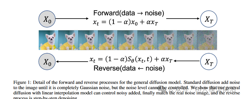
Forward Process: Starting from real data, gradually add noise until reaching a pure noise state. During this process, the noise level at each step needs to be calculated and saved. -
Reverse Process: Starting from pure noise, gradually remove noise until recovering to the target data. In this process, a neural network (usually a U-Net structure) is used to predict the noise level at each step and generate data accordingly. -
Optimization: Train the model by minimizing the difference between real data and generated data. Common loss functions include MSE (Mean Squared Error) and BCE (Binary Cross Entropy).
-
High generation quality: The Diffusion Model can generate high-quality data due to its stepwise diffusion and recovery process. -
Strong interpretability: The generation process of the Diffusion Model has clear physical meaning, making it easier to understand and explain. -
Good flexibility: The Diffusion Model can handle various types of data, including images, text, and audio.
-
Long training time: The Diffusion Model requires a lengthy training time due to the multiple steps of diffusion and recovery. -
High computational resource demand: To ensure generation quality, the Diffusion Model typically requires substantial computational resources, including memory and computational power.
import torch
import torch.nn as nn
import torch.optim as optim
# Define U-Net model
class UNet(nn.Module):
    # ... omitted model definition...
# Define Diffusion Model
class DiffusionModel(nn.Module):
    def __init__(self, unet):
        super(DiffusionModel, self).__init__()
        self.unet = unet
    def forward(self, x_t, t):
        # x_t is the data at the current moment, t is the noise level
        # Use U-Net to predict noise level
        noise_pred = self.unet(x_t, t)
        # Generate data based on noise level
        x_t_minus_1 = x_t - noise_pred * torch.sqrt(1 - torch.exp(-2 * t))
        return x_t_minus_1
# Initialize model and optimizer
unet = UNet()
model = DiffusionModel(unet)
optimizer = optim.Adam(model.parameters(), lr=0.001)
# Training process
for epoch in range(num_epochs):
    for x_real in dataloader:  # Get real data from data loader
        # Forward process
        x_t = x_real  # Start from real data
        for t in torch.linspace(0, 1, num_steps):
            # Add noise
            noise = torch.randn_like(x_t) * torch.sqrt(1 - torch.exp(-2 * t))
            x_t = x_t + noise * torch.sqrt(torch.exp(-2 * t))
            # Calculate predicted noise
            noise_pred = model(x_t, t)
            # Calculate loss
            loss = nn.MSELoss()(noise_pred, noise)
            # Backpropagation and optimization
            optimizer.zero_grad()
            loss.backward()
            optimizer.step()
About Us
Data Party THU, as a data science public account backed by the Tsinghua University Big Data Research Center, shares cutting-edge data science and big data technology innovation research dynamics, continuously disseminates data science knowledge, and strives to build a platform for gathering data talents, creating the strongest group of big data in China.

Sina Weibo: @Data Party THU
WeChat Video Account: Data Party THU
Today’s Headlines: Data Party THU