Detailed Analysis of PyTorch’s Autograd Mechanism

Click the "Little White Learns Vision" above, select "Star" or "Top"
Heavy content delivered at the first time

Author: Vaibhav Kumar

Compiled by: ronghuaiyang

We all agree that when it comes to large neural networks, we are not good at calculus. It is impractical to compute the gradients of such large composite functions by explicitly solving mathematical equations, especially when these curves exist in a vast number of dimensions that are incomprehensible.

To deal with hyperplanes in 14-dimensional space, imagine a three-dimensional space and loudly tell yourself “14.” Everyone does this – Geoffrey Hinton

This is where PyTorch’s autograd comes into play. It abstracts complex mathematics, helping us to “magically” compute the gradients of high-dimensional curves with just a few lines of code. This article attempts to describe the magic of autograd.

Basics of PyTorch

Before further discussion, we need to understand some basic PyTorch concepts.

Tensors: Simply put, it is just an n-dimensional array in PyTorch. Tensors support some additional enhancements that make them unique: in addition to CPU, they can be loaded or computed faster on GPU. When setting .requires_grad = True, they start forming a backward graph that tracks every operation applied to them, computing gradients using a so-called dynamic computation graph (DCG) (which will be explained further later).

In earlier versions of PyTorch, the torch.autograd.Variable class was used to create tensors that support gradient computation and operation tracking, but as of PyTorch v0.4.0, the Variable class has been deprecated. torch.Tensor and torch.autograd.Variable are now the same class. More accurately, torch.Tensor can track history and behaves like the old Variable.

import torch
import numpy as np

x = torch.randn(2, 2, requires_grad=True)  # From numpy
x = np.array([1., 2., 3.])  # Only Tensors of floating point dtype can require gradients
x = torch.from_numpy(x)  # Now enable gradient
x.requires_grad_(True)  # _ above makes the change in-place (it's a common PyTorch thing)

Note: According to PyTorch’s design, gradients can only be computed for floating point tensors, which is why I created a floating-point numpy array and then set it to be a PyTorch tensor with gradients enabled.

Autograd: This class is a derivative computation engine (more precisely, the Jacobian vector product). It records a graph of all operations on the gradient tensor and creates a non-cyclic graph called the dynamic computation graph. The leaf nodes of this graph are the input tensors, and the root nodes are the output tensors. Gradients are computed by tracing the graph from root to leaf and multiplying each gradient using the chain rule.

Neural Networks and Backpropagation

Neural networks are simply composite mathematical functions that have been fine-tuned (trained) to output the desired results. The adjustment or training is accomplished through an excellent algorithm called backpropagation. Backpropagation is used to compute the loss gradients with respect to input weights so that the weights can be updated later, ultimately reducing the loss.

In a way, backpropagation is just a fancy name for the chain rule – Jeremy Howard

Creating and training neural networks involves the following basic steps:

1. Define the architecture

2. Forward propagate using input data on the architecture

3. Compute the loss

4. Backpropagate, computing the gradient for each weight

5. Update the weights using the learning rate

The small changes in input weights caused by the loss change are called the gradients of that weight and are computed using backpropagation. The gradients are then used to update the weights, using the learning rate to overall reduce the loss and train the neural network.

This is done iteratively. For each iteration, several gradients are computed, and a structure called a computation graph is built to store these gradient functions. PyTorch achieves this by building a dynamic computation graph (DCG). This graph is constructed from scratch in each iteration, providing maximum flexibility for gradient computation. For example, for the forward operation (function) Mul, the backward operation function MulBackward is dynamically integrated into the backward graph to compute gradients.

Dynamic Computation Graph

Gradient-enabled tensors (variables) and functions (operations) combine to create a dynamic computation graph. The data flow and operations applied to the data are defined at runtime, dynamically constructing the computation graph. This graph is dynamically generated by the underlying autograd class. You do not have to code all possible paths before starting training – you run what you differentiate.

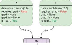
A simple DCG for the multiplication of two tensors would look like this:

Each outlined box in the graph represents a variable, while the purple rectangular boxes represent operations.

Each variable object has several members, some of which are:

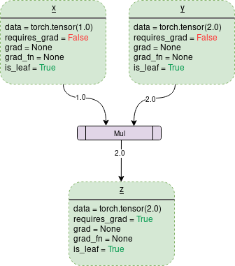
Data: It is the data held by a variable. x holds a 1×1 tensor with a value of 1.0, while y holds 2.0. z holds the product of the two, which is 2.0.

requires_grad: This member (if true) starts tracking all operation history and forms a backward graph for gradient computation. For any tensor a, it can be processed in place as follows: a.requires_grad_(True).

grad: grad holds the gradient values. If requires_grad is False, it will hold a None value. Even if requires_grad is true, it will hold a None value unless the .backward() function is called from other nodes. For example, if you compute the gradient of out with respect to x, calling out.backward() will give x.grad the value of ∂out/∂x.

grad_fn: This is the backward function used to compute gradients.

is_leaf: If:

1. It is explicitly initialized by some function, such as x = torch.tensor(1.0) or x = torch.randn(1, 1) (basically all tensor initialization methods discussed at the beginning of this article).

2. It is created after operations on a tensor, and all tensors have requires_grad = False.

3. It is created by calling the .detach() method on some tensor.

When calling backward(), only the gradients of nodes where requires_grad and is_leaf are both true are computed.

When requires_grad = True is turned on, PyTorch starts tracking operations and stores the gradient functions at each step as follows:

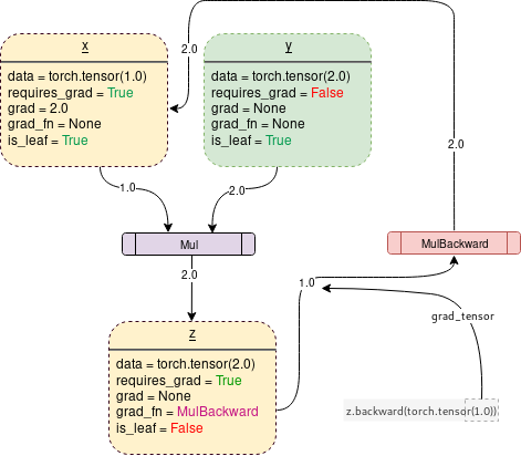
The code to generate the above figure in PyTorch is:

Backward() Function

The Backward function actually computes the gradient by passing parameters (a 1×1 unit tensor by default) through the Backward graph all the way to each leaf node, where each leaf node can trace back to the root tensor called. Remember, the backward graph has already been dynamically generated during the forward pass. The backward function only uses the generated graph to compute gradients and stores them in the leaf nodes.

Let’s analyze the following code:

import torch
# Creating the graph
x = torch.tensor(1.0, requires_grad=True)
z = x ** 3
z.backward()  # Computes the gradient
print(x.grad.data)  # Prints '3' which is dz/dx

One important thing to note is that when calling z.backward(), a tensor is automatically passed as z.backward(torch.tensor(1.0)). torch.tensor(1.0) is used to terminate the chain rule’s gradient multiplication. This external gradient is passed as an input to the MulBackward function for further computation of x‘s gradient. The dimensions of the tensor passed to .backward() must match the dimensions of the tensor for which gradients are being computed. For example, if the gradient-enabled tensors x and y are as follows:

x = torch.tensor([0.0, 2.0, 8.0], requires_grad=True)
y = torch.tensor([5.0 , 1.0 , 7.0], requires_grad=True)
z = x * y

Then, to compute the gradient of z with respect to x or y, an external gradient must be passed to the z.backward() function, as follows:

z.backward(torch.FloatTensor([1.0, 1.0, 1.0]))

z.backward() will give a RuntimeError: grad can be implicitly created only for scalar outputs

The tensor passed to the backward function acts like the weight of the gradient-weighted output. Mathematically, this is a vector multiplied by the Jacobian matrix of a non-scalar tensor (which will be further discussed in this article), so it is almost always a unit tensor of the same dimension as the backward tensor, unless a weighted output needs to be computed.

tldr: The backward graph is automatically and dynamically created by the autograd class during the forward pass. Backward() simply computes the gradients by passing its parameters to the already generated backward graph.

Mathematics – Jacobian Matrix and Vector

Mathematically, the autograd class is just a Jacobian vector product computation engine. The Jacobian matrix is a very simple word that represents all possible partial derivatives between two vectors. It is the gradient of one vector with respect to another vector.

Note: In this process, PyTorch never explicitly constructs the entire Jacobian matrix. Direct computation of JVP (Jacobian vector product) is usually simpler and more efficient.

If a vector X = [x1, x2, …xn] computes another vector through f(X) = [f1, f2, …fn], then the Jacobian matrix (J) contains all combinations of partial derivatives as follows:

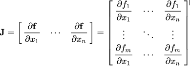
The above matrix represents the gradient of f(X) with respect to X.

Assuming a tensor X with PyTorch gradients enabled:

X = [x1,x2,…,xn] (assuming this is the weights of some machine learning model)

X forms a vector Y through some operations

Y = f(X) = [y1, y2,…,ym]

Then using Y to compute a scalar loss l. Assuming the vector v is exactly the gradient of the scalar loss l with respect to the vector Y as follows:

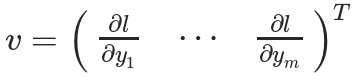
The vector v is called grad_tensor and is passed as a parameter to the backward() function.

To obtain the gradient of the loss l with respect to the weights X, the Jacobian matrix J is the vector multiplied by the vector v

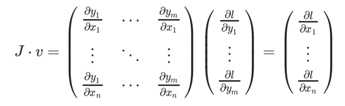
This method of computing the Jacobian matrix and multiplying it by the vector v allows PyTorch to easily provide external gradients for non-scalar outputs.

Good news!
Little White Learns Vision knowledge circle
Now open to the outside👇👇👇



Download 1: OpenCV-Contrib Extension Module Chinese Version Tutorial
Reply "Extension Module Chinese Tutorial" in the backend of "Little White Learns Vision" public account to download the first OpenCV extension module tutorial in Chinese, covering installation of extension modules, SFM algorithms, stereo vision, object tracking, biological vision, super-resolution processing, etc., with more than twenty chapters of content.

Download 2: Python Vision Practical Project 52 Lectures
Reply "Python Vision Practical Project" in the backend of "Little White Learns Vision" public account to download 31 vision practical projects including image segmentation, mask detection, lane line detection, vehicle counting, adding eyeliner, license plate recognition, character recognition, emotion detection, text content extraction, facial recognition, etc., to help quickly learn computer vision.

Download 3: OpenCV Practical Project 20 Lectures
Reply "OpenCV Practical Project 20 Lectures" in the backend of "Little White Learns Vision" public account to download containing 20 practical projects based on OpenCV, achieving advanced learning of OpenCV.

Discussion Group

Welcome to join the reader group of the public account to communicate with peers. Currently, there are WeChat groups for SLAM, 3D vision, sensors, autonomous driving, computational photography, detection, segmentation, recognition, medical imaging, GAN, algorithm competitions, etc. (will gradually be subdivided in the future). Please scan the WeChat ID below to join the group, with the note: "Nickname + School/Company + Research Direction", for example: "Zhang San + Shanghai Jiao Tong University + Vision SLAM". Please follow the format for remarks, otherwise, it will not be approved. After successful addition, you will be invited to enter the relevant WeChat group according to your research direction. Please do not send advertisements in the group, otherwise, you will be removed from the group. Thank you for your understanding~