TensorFlow 2.x offers a lot of simplicity in building models and overall use of TensorFlow. So what are the new changes in TF2?

• Use Keras to easily build models and execute immediately.
• Powerful model deployment on any platform.
• Robust research experiments.
• Simplified API by cleaning up deprecated APIs and reducing redundancy.

In this article, we will explore 10 features of TF 2.0 that make using TensorFlow smoother, reduce the number of lines of code, and improve efficiency.

1(a). tf.data Building Input Pipelines

tf.data provides functionalities for data pipelines and related operations. We can build pipelines, map preprocessing functions, shuffle or batch datasets, and more.

Building Pipelines from Tensors

>>> dataset = tf.data.Dataset.from_tensor_slices([8, 3, 0, 8, 2, 1])
>>> iter(dataset).next().numpy()
8

Building Batches and Shuffling

# Shuffle
>>> dataset = tf.data.Dataset.from_tensor_slices([8, 3, 0, 8, 2, 1]).shuffle(6)
>>> iter(dataset).next().numpy()
0

# Batch
>>> dataset = tf.data.Dataset.from_tensor_slices([8, 3, 0, 8, 2, 1]).batch(2)
>>> iter(dataset).next().numpy()
array([8, 3], dtype=int32)

# Shuffle and Batch
>>> dataset = tf.data.Dataset.from_tensor_slices([8, 3, 0, 8, 2, 1]).shuffle(6).batch(2)
>>> iter(dataset).next().numpy()
array([3, 0], dtype=int32)

Compressing Two Datasets into One

>>> dataset0 = tf.data.Dataset.from_tensor_slices([8, 3, 0, 8, 2, 1])
>>> dataset1 = tf.data.Dataset.from_tensor_slices([1, 2, 3, 4, 5, 6])
>>> dataset = tf.data.Dataset.zip((dataset0, dataset1))
>>> iter(dataset).next()
(<tf.tensor: dtype="int32," numpy="8" shape="(),">, <tf.tensor: dtype="int32," numpy="1" shape="(),">)
</tf.tensor:></tf.tensor:>

Mapping External Functions

def into_2(num):
     return num * 2
    
>>> dataset = tf.data.Dataset.from_tensor_slices([8, 3, 0, 8, 2, 1]).map(into_2)
>>> iter(dataset).next().numpy()
16

1(b). ImageDataGenerator

This is one of the best features of the tensorflow.keras API. ImageDataGenerator can generate dataset slices in real-time while batching, preprocessing, and augmenting data.

The generator allows for data streams directly from directories or data directories.

One misconception about data augmentation in ImageDataGenerator is that it adds more data to the existing dataset. While this is the actual definition of data augmentation, in ImageDataGenerator, the images in the dataset are dynamically transformed during different steps of training, allowing the model to train on unseen noisy data.

train_datagen = ImageDataGenerator(
        rescale=1./255,
        shear_range=0.2,
        zoom_range=0.2,
        horizontal_flip=True
)

Here, all samples are rescaled (for normalization), while other parameters are used for augmentation.

train_generator = train_datagen.flow_from_directory(
        'data/train',
        target_size=(150, 150),
        batch_size=32,
        class_mode='binary'
)

We specify the directory for the real-time data stream. This can also be done using dataframes.

train_generator = flow_from_dataframe(
    dataframe,
    x_col='filename',
    y_col='class',
    class_mode='categorical',
    batch_size=32
)

The x_col parameter defines the full path of the image, while the y_col parameter defines the label column for classification.

The model can be fed data directly from the generator. The steps_per_epoch parameter needs to be specified, which is number_of_samples // batch_size.

model.fit(
    train_generator,
    validation_data=val_generator,
    epochs=EPOCHS,
    steps_per_epoch=(num_samples // batch_size),
    validation_steps=(num_val_samples // batch_size)
)

2. Using tf.image for Data Augmentation

Data augmentation is necessary. In cases of insufficient data, modifying data and treating it as separate data points is a very effective way to train with less data.

The tf.image API has tools for transforming images, which can then be used for data augmentation with tf.data.

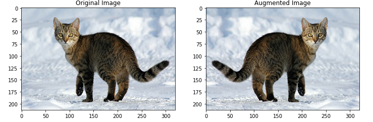
flipped = tf.image.flip_left_right(image)
visualise(image, flipped)

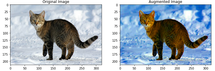
saturated = tf.image.adjust_saturation(image, 5)
visualise(image, saturated)

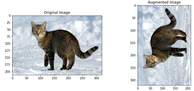
rotated = tf.image.rot90(image)
visualise(image, rotated)

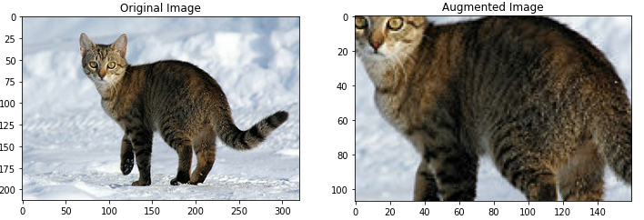
cropped = tf.image.central_crop(image, central_fraction=0.5)
visualise(image, cropped)

3. TensorFlow Datasets

pip install tensorflow-datasets

This is a very useful library as it contains very well-known datasets collected by TensorFlow from various domains.

import tensorflow_datasets as tfds

mnist_data = tfds.load("mnist")
mnist_train, mnist_test = mnist_data["train"], mnist_data["test"]
assert isinstance(mnist_train, tf.data.Dataset)

A detailed list of datasets available in tensorflow-datasets can be found at: https://www.tensorflow.org/datasets/catalog/overview.

The types of datasets provided by tfds include: audio, image, image classification, object detection, structured data, summarization, text, translation, video.

4. Using Pre-trained Models for Transfer Learning

Transfer learning is a new technique in machine learning that is very important. If a benchmark model has already been trained by someone else, and training it requires a lot of resources (e.g., multiple expensive GPUs that one might not afford), transfer learning solves this problem. Pre-trained models can be reused in specific scenarios or expanded for different scenarios.

TensorFlow provides benchmark pre-trained models that can be easily expanded for the desired scenarios.

base_model = tf.keras.applications.MobileNetV2(
    input_shape=IMG_SHAPE,
    include_top=False,
    weights='imagenet'
)

This base_model can be easily expanded with additional layers or different models, such as:

model = tf.keras.Sequential([
    base_model,
    global_average_layer,
    prediction_layer
])

5. Estimators

Estimators are a high-level representation of complete models in TensorFlow, designed for easy scalability and asynchronous training.

Predefined estimators provide a very high-level model abstraction so you can focus directly on training the model without worrying about the underlying complexities. For example:

linear_est = tf.estimator.LinearClassifier(
    feature_columns=feature_columns
)

linear_est.train(train_input_fn)
result = linear_est.evaluate(eval_input_fn)

This demonstrates how easy it is to build and train an estimator using tf.estimator. Estimators can also be customized.

TensorFlow has many estimators, including LinearRegressor, BoostedTreesClassifier, etc.

6. Custom Layers

Neural networks are known for their many layers deep architecture, where layers can be of different types. TensorFlow includes many predefined layers (such as density, LSTM, etc.). However, for more complex architectures, the logic of the layers can be much more complex than basic layers. For such cases, TensorFlow allows building custom layers. This can be done by subclassing tf.keras.layers.

class CustomDense(tf.keras.layers.Layer):
    def __init__(self, num_outputs):
        super(CustomDense, self).__init__()
        self.num_outputs = num_outputs

    def build(self, input_shape):
        self.kernel = self.add_weight(
            "kernel",
            shape=[int(input_shape[-1],
            self.num_outputs]
        )

    def call(self, input):
        return tf.matmul(input, self.kernel)

As stated in the documentation, the best way to implement your own layer is to extend the tf.keras.Layer class and implement:

1. __init__, where you can do all initialization unrelated to input.
2. build, where you know the shape of the input tensor and can do the remaining initialization work.
3. call, where the forward computation is done.

While kernel initialization can be done in __init__, it is better to do it in build, otherwise you have to explicitly specify input_shape for every instance of the new layer.

7. Custom Training

tf.keras Sequential and Model API make training models easier. However, most of the time when training complex models, using custom loss functions is necessary. Additionally, model training may differ from the default training (e.g., calculating gradients separately for different model components).

TensorFlow’s automatic differentiation helps to compute gradients efficiently. These primitives are used to define custom training loops.

def train(model, inputs, outputs, learning_rate):
    with tf.GradientTape() as t:
        # Computing Losses from Model Prediction
        current_loss = loss(outputs, model(inputs))
        
    # Gradients for Trainable Variables with Obtained Losses
    dW, db = t.gradient(current_loss, [model.W, model.b])
    
    # Applying Gradients to Weights
    model.W.assign_sub(learning_rate * dW)
    model.b.assign_sub(learning_rate * db)

This loop can be repeated across multiple epochs and can use more customized settings based on the use case.

8. Checkpoints

There are two ways to save a TensorFlow model:

1. SavedModel: Saves the complete state of the model along with all parameters. This is independent of the source code.<span>model.save_weights('checkpoint')</span>
2. Checkpoints

Checkpoints capture the values of all parameters used by the model. Models built using the Sequential API or Model API can simply be saved in the SavedModel format.

However, for custom models, checkpoints are required.

Checkpoints do not contain any description of the computations defined by the model, so saved parameter values are usually useful only when the source code is available.

Saving Checkpoints

checkpoint_path = "save_path"

# Defining a Checkpoint
ckpt = tf.train.Checkpoint(model=model, optimizer=optimizer)

# Creating a CheckpointManager Object
ckpt_manager = tf.train.CheckpointManager(ckpt, checkpoint_path, max_to_keep=5)

# Saving a Model
ckpt_manager.save()

Loading Model from Checkpoint

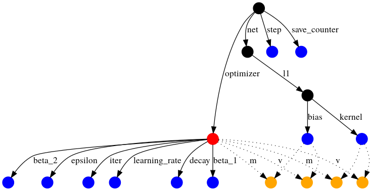
TensorFlow starts from the loaded object, matching variables with checkpoint values by traversing the directed graph with named edges.

if ckpt_manager.latest_checkpoint:
    ckpt.restore(ckpt_manager.latest_checkpoint)

9. Keras Tuner

This is a relatively new feature in TensorFlow.

!pip install keras-tuner

Hyperparameter tuning is the process of screening parameters defined for the configuration of ML models. After feature engineering and preprocessing, these factors are decisive for model performance.

# model_builder is a function that builds a model and returns it
tuner = kt.Hyperband(
    model_builder,
    objective='val_accuracy', 
    max_epochs=10,
    factor=3,
    directory='my_dir',
    project_name='intro_to_kt'
)

In addition to HyperBand, Bayesian Optimization and Random Search can also be used for tuning.

tuner.search(
    img_train, label_train, 
    epochs = 10, 
    validation_data=(img_test,label_test), 
    callbacks=[ClearTrainingOutput()]
)

# Get the optimal hyperparameters
best_hps = tuner.get_best_hyperparameters(num_trials=1)[0]

Then, we train the model using the optimal hyperparameters:

model = tuner.hypermodel.build(best_hps)
model.fit(
    img_train, 
    label_train, 
    epochs=10, 
    validation_data=(img_test, label_test)
)

10. Distributed Training

If you have multiple GPUs and want to optimize training across multiple GPUs through distributed training loops, TensorFlow’s various distributed training strategies can optimize GPU usage and manage training on GPUs for you.

tf.distribute.MirroredStrategy is the most commonly used strategy. How does it work?

• All variables and model graphs are duplicated into copies.
• Inputs are evenly distributed across different copies.
• Each copy computes the loss and gradients for the inputs it receives.
• Gradients of all copies are synchronized and summed.
• After synchronization, the same updates are applied to the variables on each copy.

strategy = tf.distribute.MirroredStrategy()with strategy.scope():
    model = tf.keras.Sequential([
        tf.keras.layers.Conv2D(
            32, 3, activation='relu',  input_shape=(28, 28, 1)
        ),
        tf.keras.layers.MaxPooling2D(),
        tf.keras.layers.Flatten(),
        tf.keras.layers.Dense(64, activation='relu'),
        tf.keras.layers.Dense(10)
    ])

    model.compile(
        loss="sparse_categorical_crossentropy",
        optimizer="adam",
        metrics=['accuracy']
    )