Diffusion models are very popular, and their descriptions vary widely. In this article, a DeepMind research scientist provides a comprehensive analysis of the topic “What is a diffusion model?”
If you’ve tried one of the most popular AI painting tools, Stable Diffusion, then you’ve already experienced the powerful generative capabilities of diffusion models. But if you want to go further and understand how they work, you’ll find that there are many forms of diffusion models.
If you randomly select two research papers on diffusion models and look at the descriptions of model categories in their introductions, you may find their descriptions vary greatly. This can be both frustrating and enlightening: frustrating because it makes it harder to see the relationship between papers and implementations, and enlightening because each perspective reveals new connections and sparks new ideas.
Recently, DeepMind research scientist Sander Dieleman published a lengthy blog post summarizing his views on diffusion models.
This article is a further extension of his previous work titled “Diffusion Models are Autoencoders” written last year. The title has a humorous undertone but emphasizes the close relationship between diffusion models and autoencoders. He believes that people still underestimate this connection.
Interested readers can visit: https://sander.ai/2022/01/31/diffusion.html
In this new article, Dieleman analyzes diffusion models from several different perspectives, including viewing diffusion models as autoencoders, deep latent variable models, models for predicting score functions, solving reverse stochastic differential equations, flow models, recurrent neural networks, autoregressive models, and models for estimating expectations. He also shares his views on the current state of research directions in diffusion models.
Diffusion Models as Autoencoders
Denoising autoencoders are a type of neural network where the input is corrupted by noise, and their task is to predict the clean input, effectively removing the corruption. To accomplish this task well, it is necessary to learn the distribution of clean data. They are very commonly used representation learning methods, and in the early development of deep learning, they were also used for layer-wise pretraining of deep neural networks.
It turns out that the neural networks used in diffusion models often solve a very similar problem: given an input example corrupted by noise, they predict some quantity related to its data distribution. This can be the corresponding clean input (like a denoising autoencoder), the noise added, or something in between (which will be detailed later). When the corruption process is linear, all of these are equivalent, meaning that if noise is added, we can simply subtract the predicted result from the noisy input, and we can turn the model predicting noise into one predicting clean input. In neural network terms, this means adding a residual connection from input to output.
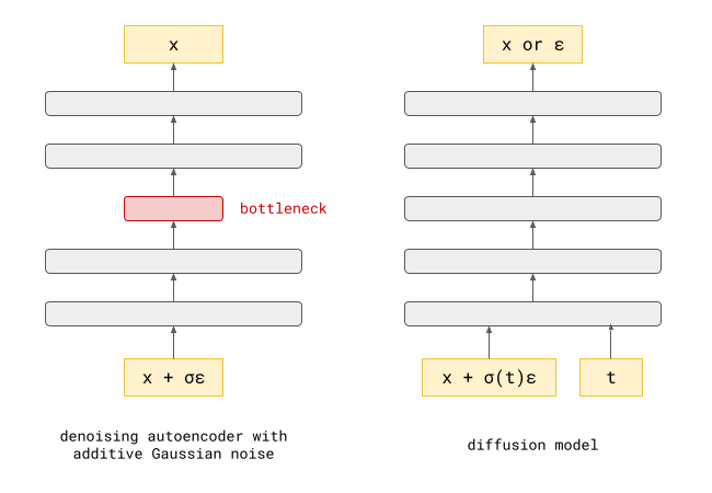
Diagram of Denoising Autoencoders (left) and Diffusion Models (right)
They have several key differences:
-
In learning useful representations of the input, there is often some information bottleneck in the middle of a denoising autoencoder that limits its ability to learn representations. The denoising task itself is just a means to an end, not the actual purpose for which we use the model after training. Neural networks used for diffusion models usually do not have such bottlenecks because we care more about their predictive results than the internal representation methods used to obtain those results.
-
Denoising autoencoders can be trained using various types of noise. For example, we can mask part of the input (masking noise), or we can add noise from some arbitrary distribution (usually Gaussian). For diffusion models, we typically stick to adding Gaussian noise because it has useful mathematical properties that simplify many operations.
-
Another important difference is that the training objective of a denoising autoencoder only deals with a specific strength of noise. In using diffusion models, we want to predict something based on inputs with varying levels of noise. The noise level is also an input to the neural network.
In fact, the author has previously discussed the relationship between the two in detail; interested readers can visit: https://sander.ai/2022/01/31/diffusion.html
Diffusion Models as Deep Latent Variable Models
Sohl-Dickstein et al. were the first to suggest using diffusion processes to gradually damage the structure of the data in a paper presented at ICML 2015, and then to learn to reverse that process to build generative models. Five years later, Ho et al. developed the Denoising Diffusion Probabilistic Model (DDPM) based on this, which, together with score-based models, forms the blueprint for diffusion models.
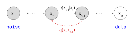
DDPM Diagram
As shown in the figure above, x_T (latent) represents Gaussian noise, while x_0 (observed) represents the data distribution. These random variables are connected by a finite number of intermediate latent variables x_t (usually T=1000), forming a Markov chain, where x_{t-1} depends only on x_t and does not directly depend on any previous random variables in the chain.
The fitting of the parameters of this Markov chain is done using variational inference to reverse the diffusion process, which is also a Markov chain (in the opposite direction, represented in the figure as q (x_t∣x_{t−1})), but this chain gradually adds Gaussian noise to the data.
Specifically, just like in Variational Autoencoders (VAEs), we can write down an evidence lower bound (ELBO), which is a bound on the log-likelihood that can be easily maximized. In fact, the subtitle of this section could also be “Diffusion Models are Deep VAEs,” but since we have already written “Diffusion Models are Autoencoders” from another perspective, we chose the current subtitle to avoid confusion.
We know that q (x_t∣x_{t−1}) is a Gaussian distribution, but the model we want to fit, p (x_{t−1}∣x_t), does not need to be. However, it turns out that as long as each individual step is small enough (i.e., T is large enough), we can set the parameters such that p (x_{t−1}∣x_t) looks like a Gaussian distribution, and its approximation error will be small enough that the model can still generate high-quality samples. This is somewhat surprising because any errors during sampling could accumulate with T.
Diffusion Models Predict Score Functions
Most likelihood-based generative models parameterize the log-likelihood log p (x∣θ) of the input x, and then fit the model parameters θ to maximize it, either by approximating (like VAEs) or exactly (like flow models or autoregressive models). Since the log-likelihood represents a probability distribution, and probability distributions must be normalized, some constraints are usually needed to ensure that all possible values of parameters θ produce valid distributions. For example, autoregressive models ensure this through causal masking, while most flow models require reversible neural network architectures.
Research shows that there is another way to fit distributions that cleverly avoids the normalization requirement, which is score matching. This is based on the observation that the so-called score function (score matching) 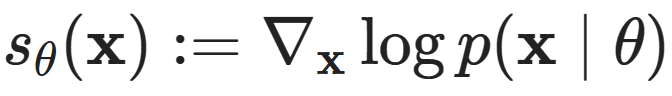 does not change with the scaling of p (x∣θ).This is easy to see:
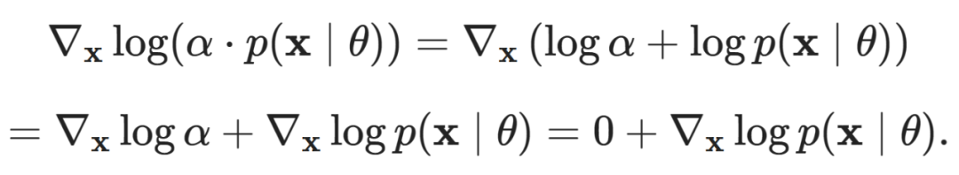
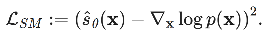
Any scaling factor applied to the probability density will disappear. Therefore, if we have a model parameterizing a direct score estimate 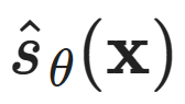 we can fit the distribution by minimizing the score matching loss (rather than directly maximizing the likelihood):
However, using this form, the loss function may not be practical because we do not have a good way to compute the true score for any data point x 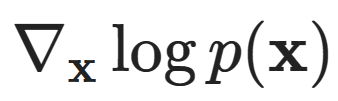 of good quality.There are some tricks available to bypass this requirement and convert it into an easily computable loss function, including implicit score matching (ISM), slice score matching (SSM), and denoising score matching (DSM). Here we will take a closer look at the last method:

Where we can obtain  by adding Gaussian noise to x.This means that
 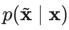 is distributed based on a Gaussian distribution N (x,σ^2), whose true conditional score function can be computed in closed form:
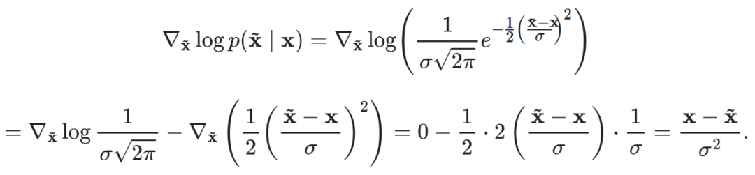
This form has a very intuitive explanation: it is an extended version of adding noise to x to obtain  . Thus, by maximizing the likelihood (which is the gradient of the log-likelihood) for
  it directly corresponds to removing (some) noise:
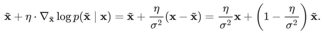
If we choose the step size η=σ^2, we can recover the clean data x in one step.
L_SM and L_DSM are different loss functions, but the clever part is that they have the same expected minimum:
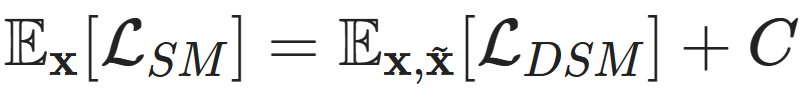 , where C is a constant.Pascal Vincent derived this equivalence back in 2010, and if you want to deepen your understanding, I highly recommend reading his technical report:http://www.iro.umontreal.ca/~vincentp/Publications/smdae_techreport.pdf
This method raises an important question: how much noise should we add, i.e., what should σ be? Choosing a fixed value for this hyperparameter does not work well in practice. At low noise levels, accurately estimating scores in low-density regions is very difficult. At high noise levels, this is not a problem because the added noise spreads across the density in all directions — then the distribution we are modeling becomes significantly distorted by the noise. A good approach is to model the density at many different noise levels. Once we have such a model, we can anneal σ during the sampling process — starting with a lot of noise and gradually decreasing it. Song & Ermon detailed these issues and proposed this elegant solution in their 2019 paper.
This method effectively combines denoising score matching at various noise levels with gradually annealing noise during sampling, resulting in a model that is essentially equivalent to DDPM, but the derivation process is entirely different — the ELBO is completely invisible!
For more detailed discussion of this method, please refer to the blog of one of the authors, Yang Song: https://yang-song.net/blog/2021/score/
Diffusion Models Solve Reverse Stochastic Differential Equations
The first two perspectives on diffusion models (deep latent variable models and score matching) consider discrete and finite steps. These steps correspond to different levels of Gaussian noise, and we can write a monotonic mapping σ(t) that indexes the steps to the standard deviation of the noise at that step.
If we let the number of steps approach infinity, we can replace these discrete index variables with continuous values t over the interval [0,T], which can be interpreted as a time variable, meaning that σ(t) now describes the evolution of the standard deviation of the noise over time. In continuous time, we can describe the diffusion process of gradually adding noise to the data point x using the following stochastic differential equation (SDE):
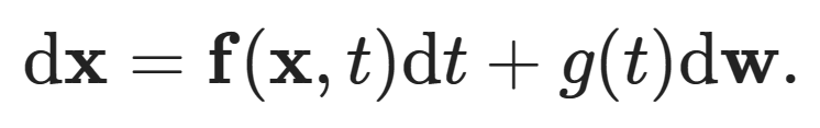
This equation relates the infinitesimal change in x to the infinitesimal change in t, where dw represents infinitesimal Gaussian noise, also known as the Wiener process. f and g are referred to as the drift coefficient and diffusion coefficient, respectively. The specific choices of f and g can yield the continuous-time version of the Markov chain used to construct DDPM.
The SDE combines differential equations and random variables, which may seem daunting at first glance. Fortunately, we do not need too many existing advanced SDE mechanisms to understand how this perspective can be applied to diffusion models. However, there is a very important result available to us. Given an SDE that describes the diffusion process as above, we can write another SDE that describes the process in the opposite direction, i.e., reversing time:

This equation also describes a diffusion process.
 is the reverse Wiener process, and
 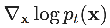 is a time-dependent score function.This time dependency arises from the fact that the noise level varies with time.
Explaining the reasons for this situation is beyond the scope of this article; interested readers can refer to the original paper by Yang Song et al. that introduced the SDE-based formalism for diffusion models, titled “Score-Based Generative Modeling through Stochastic Differential Equations”.
Specifically, if we have a method to estimate the time-dependent score function, we can simulate the reverse diffusion process to extract samples from the data distribution that starts with noise. We can again train a neural network to predict this quantity and insert it into the reverse SDE to obtain a continuous-time diffusion model.
In practice, simulating this SDE requires discretizing the time variable t again, so you might wonder why we would do this. The clever part is that now we can decide the discretization at the sampling time, and we do not have to fix it before we have trained the score prediction model. In other words, by choosing the number of sampling steps, we can naturally balance the sampling quality and computational cost without modifying the model.
Diffusion Models as Flow Models
Remember flow models? Flow models are not commonly used generative models today, mainly because they require more parameters to match the performance of other models. This is due to their limited expressiveness: the neural networks used in flow models need to be reversible, and the log determinant of their Jacobian must be easy to compute, which severely limits the types of computations possible.
At least this is the case for discrete normalized flows. Continuous normalized flows (CNF) also exist, and their usual form is a deterministic path described by an ordinary differential equation (ODE) parameterized by neural networks, which describes the correspondence between samples in the data distribution and samples from a simple base distribution. CNF is not affected by the constraints of the neural network architectures mentioned earlier, but its original form requires training with backpropagation through an ODE solver. While some tricks can be used to accomplish this more efficiently, it can still hinder wider adoption.
Let’s revisit the SDE formalism of diffusion models, which describes a stochastic process mapping samples from a simple base distribution to samples from the data distribution. An interesting question arises: what is the distribution of the intermediate samples p_t (x), and how does it change over time? This is governed by the Fokker-Planck equation. If you want to understand the practical implications, check out Appendix D.1 of the paper by Song et al. (2021).
Here comes the crazy part: the time-dependent distribution described by an ODE corresponds exactly to the stochastic process described by this SDE! This is called the probability flow ODE. Moreover, it has a simple closed-form:
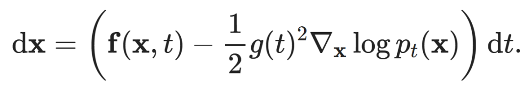
This equation describes both the forward and backward processes (simply change the sign to switch directions), and note that the time-dependent score function 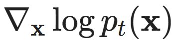 is still present.To prove this, you can write down the Fokker-Planck equations for both the SDE and the probability flow ODE, and do some algebra, and you will find that they are indeed the same, thus must have the same solution p_t (x).
Please note that the process described by this ODE is not the same as that described by this SDE, which cannot be the case because deterministic differential equations cannot describe a stochastic process. It describes a different process with a unique property: the distributions p_t (x) of the two processes are the same.
This phenomenon reveals important significance: there exists a bijective mapping between specific samples from the simple base distribution and samples from the data distribution. For the sampling process where all randomness is contained in the initial base distribution sample — once the sampling is complete, the process of obtaining data samples based on this is completely deterministic. This also means that we can map data points to their corresponding latent representations by forward simulating the ODE, manipulate them, and then map them back to data space by backward simulating the ODE.
The model described by this probability flow ODE is a continuous normalized flow model, but we can train it without backpropagating through the ODE, making the scalability of this method much better.
Isn’t it amazing that we can do this without changing the way the model is trained? We can insert the score predictor into either the reverse SDE mentioned in the previous section or the ODE of this section, yielding two different generative models modeling the same distribution in different ways. Isn’t that cool?
Moreover, the probability flow ODE also allows diffusion models to perform likelihood calculations, as seen in Appendix D.2 of Song et al. (2021). This also requires solving the ODE, so the cost is nearly as high as sampling.
For these reasons, the probability flow ODE paradigm has recently become quite popular. For example, Karras et al. used it as a basis to explore different design choices for diffusion models, and the author also used it in their diffusion language model with collaborators. This has also been generalized and extended beyond the diffusion process to learn mappings between arbitrary pairs of distributions, including flow matching, rectified flows, and stochastic interpolants.
As a side note, DDIM provides another way to obtain a deterministic sampling process for diffusion models based on the deep latent variable model perspective.
Diffusion Models as Recurrent Neural Networks (RNN)
Sampling from diffusion models involves repeatedly making predictions using neural networks and using those predictions to update a “canvas,” which initially consists entirely of random noise. If we consider the complete computation graph of this process, it looks very much like a recurrent neural network (RNN). In an RNN, there is a hidden state that is updated repeatedly through a recurrent unit, which consists of one or more nonlinear parameterized operations (like the gating mechanism of LSTM). Here, the hidden state is the canvas, so it lies in the input space, and its units are formed by the denoising neural networks we trained for the diffusion model.
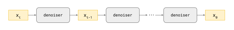
Diagram of Expanded Diffusion Sampling Loop
Training RNNs typically uses backpropagation through time (BPTT), where gradients are propagated through the recurrence. The number of recurrent steps through which backpropagation occurs is usually limited to a maximum value to reduce computational costs, known as truncated BPTT. Diffusion models are also trained through backpropagation, but only one step at a time. In a sense, diffusion models provide a way to train deep recurrent neural networks without having to backpropagate through the recurrence, thus allowing for a more scalable training process.
RNNs are usually deterministic, so this analogy is most meaningful for the deterministic process based on the probability flow ODE described in the previous section — although injecting noise into the hidden state of the RNN as a form of regularization is not unheard of, so the author believes this analogy also applies to stochastic processes.
In terms of the number of nonlinear layers, the total depth of this computation graph is given by the number of layers in the neural network multiplied by the number of sampling steps. We can think of the expanded recurrence as a very deep neural network, potentially having thousands of layers. The depth is large, but it makes sense because generative modeling of real-world data requires such a deep computation graph.
We can also think about what would happen if we did not use the same neural network at each diffusion sampling step, but instead used different neural networks for different ranges of noise levels. These networks could be trained independently and even use different architectures. This means we could effectively “unroll” the weights in a very deep neural network, turning it from an RNN into a traditional deep neural network, but we still could not avoid backpropagating through all of them at once. Stable Diffusion XL achieved great results using this method in its Refiner model, so the popularity of this method may catch on.
The author notes that when he started his PhD in 2010, training neural networks with more than 2 hidden layers was a tedious task: backpropagation was not easy to use, so their approach was to use unsupervised layer-wise pretraining to find a good initialization that made backpropagation feasible. Nowadays, even with hundreds of hidden layers, it is no longer an obstacle. Therefore, it is not difficult to imagine that in the coming years, training neural networks with thousands of layers using backpropagation could also become feasible. By then, the “divide and conquer” approach offered by diffusion models may lose its luster, and perhaps we will all return to training deep variational autoencoders! (Note that the same “divide and conquer” perspective also applies to autoregressive models, so if this does happen in the future, autoregressive models may also become obsolete.)
One question from this perspective is: would the performance of diffusion models improve if we backpropagate through the sampling process for two steps or more? This method is not common, which may indicate that it is practically costly to implement. However, there is an important exception (to some extent), models like recurrent interface networks (RIN) that use self-conditioning not only pass the updated canvas between diffusion sampling steps but also pass some form of state. To help the model learn to use this state, an approximate value of the state can be provided during training by running extra forward passes. However, there will be no additional backward passes, so this does not actually count as two-step BPTT — it’s more like 1.5 steps.
Diffusion Models as Autoregressive Models
For diffusion models of natural images, the sampling process often first produces large-scale structures and then iteratively adds finer details. In fact, there seems to be an almost direct correspondence between noise levels and feature scales.
But why is that? To understand this, thinking from the perspective of spatial frequency can be helpful. Large-scale features in images correspond to low spatial frequencies, while fine-grained details correspond to high frequencies. We can use 2D Fourier transforms (or some variant) to decompose an image into its spatial frequency components. This is often the first step in image compression algorithms, as it is well known that the human visual system is less sensitive to high frequencies, allowing for more compression of high frequencies and less compression of low frequencies.
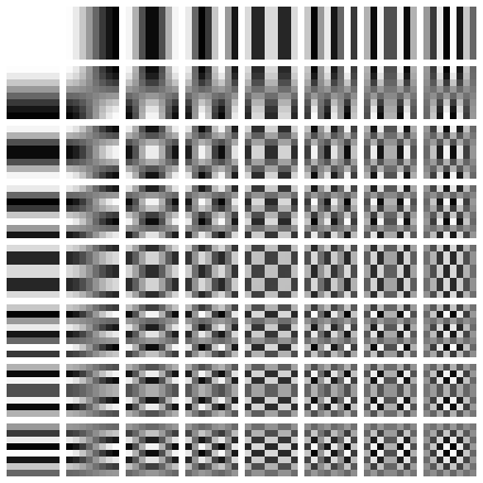
Visualization of Spatial Frequency Components of 8×8 Discrete Cosine Transform (for example, JPEG compression methods use this)
Natural images and many other natural signals exhibit an interesting phenomenon in the frequency domain: the amplitude of different frequency components often decreases proportionally with the inverse of the frequency: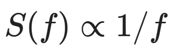 (if you are looking at the power spectrum instead of the amplitude spectrum, then it is the inverse square of the frequency).
On the other hand, the spectrum of Gaussian noise is flat: on average, the amplitudes are the same across frequencies. Since the Fourier transform is a linear operation, adding Gaussian noise to a natural image produces a new image whose frequency spectrum is the sum of the original image’s spectrum and the flat spectrum of the noise. In the logarithmic domain, the superposition of the two spectra looks like a hinge, indicating that adding noise will blur any structures present in the higher spatial frequencies in some way (see the figure below). The larger the standard deviation of this noise, the more spatial frequencies are affected.
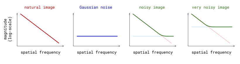
Amplitude Spectra of Natural Images, Gaussian Noise, and Noisy Images
Since diffusion models are constructed by gradually adding more noise to the input samples, we can say that this process gradually drowns out increasingly lower frequency content until all structure is eliminated (at least for natural images). When sampling from the model, the process is reversed, effectively adding structure at increasingly higher spatial frequencies. This is essentially the same as autoregression, but in frequency space! Rissanen et al. (2023) discussed this phenomenon they observed in generative modeling using reverse heat dissipation (a method that is an alternative to Gaussian diffusion), but they did not connect it to autoregressive models. This connection is proposed by the author of this article and may be controversial.
An important caveat is that this explanation relies on the frequency characteristics of natural signals, so this analogy may not hold for applications of diffusion models in other domains, such as language modeling.
Diffusion Models Estimate Expectations
The transition density p (x_t∣x_0) describes: based on the original clean input x_0, the distribution of the noisy data example x_t derived from it (by adding noise) at time t. The task of the neural networks in diffusion models is to predict its expectation E [x_0∣x_t] (or some linear time-dependent function of the expectation) based on samples from this distribution. This may seem obvious, but it also illustrates something important, so let’s emphasize it.
First, this provides evidence that using mean squared error (MSE) as the loss function when training diffusion models is the correct choice. During training, the expectation E [x_0∣x_t] is unknown, so we supervise the model using x_0 itself. Because the minimum of the MSE loss is precisely the expected value, we can ultimately recover an approximation of E [x_0∣x_t], even if we did not know this quantity in advance. This is somewhat different from a typical supervised learning problem. In a typical supervised learning problem, the ideal outcome is for the model to accurately predict the target used for supervision (excluding any labeling errors). Here, we deliberately do not want that. More generally, the concept of estimating conditional expectations (even if we are just providing supervision through samples) is very powerful.
In fact, this explains why distilling diffusion models is such an appealing proposition: in this case, we can directly use the approximate value of the target expectation E [x_0∣x_t] we want to predict to supervise the diffusion model, as the teacher model has already provided it. The result is that the variance of its training loss will be much lower than when training from scratch, and the convergence will be much faster. Of course, this is only useful if you already have a trained model available to serve as a teacher.
Discrete and Continuous Diffusion Models
So far, we have considered cases with several discrete noise levels from several perspectives, and there are also several perspectives that use continuous time concepts, which, combined with the mapping function σ(t), can map time steps to the corresponding standard deviations of noise. These are usually referred to as discrete time or continuous time, respectively. One very clever thing is that this is mainly a matter of interpretation: models trained under a discrete time perspective can usually be easily repurposed to work in a continuous time setting, and vice versa.
Another way to look at whether diffusion models are discrete or continuous is to look at the input space. The author finds that the literature often does not clearly state whether “continuous” or “discrete” is relative to time or to input. This is very important because some perspectives only make sense for continuous inputs, as they rely on gradients of the inputs (i.e., all perspectives based on score functions).
There are four combinations of discreteness/continuity:
-
Time discrete, input continuous: original deep latent variable model perspective (DDPM) and score-based perspective;
-
Time continuous, input continuous: perspectives based on SDE and ODE;
-
Time discrete, input discrete: D3PM, MaskGIT, Mask-predict, ARDM, polynomial diffusion, and SUNDAE all use iterative refinement methods for discrete inputs — whether all these should be considered diffusion models is not entirely clear (it depends on whom you ask);
-
Time continuous, input discrete: continuous-time Markov chains (CTMC), score-based continuous-time discrete diffusion models, and Blackout Diffusion all pair discrete inputs with continuous time — the usual handling of this setup is to embed discrete data into Euclidean space and then perform continuous diffusion on the inputs in that space, such as Analog Bits, Self-conditioned Embedding Diffusion, and CDCD.
Other Forms
Recently, some papers have proposed new derivations for these types of models based on first principles, completely avoiding differential equations, ELBO, or score matching due to hindsight. However, these studies provide another perspective on diffusion models, which may be easier to understand as they require less background knowledge.
Inversion by Direct Iteration (InDI) is rooted in image restoration, aiming to improve perceptual quality through iterative refinement. It makes no assumptions about the nature of image degradation, and the model is trained using paired low-quality and high-quality samples. Iterative α-(de) blending obtains a deterministic mapping between two distributions by starting with linear interpolation between samples from two different distributions. Both methods are closely related to the previously discussed flow matching, rectified flows, and stochastic interpolants.
Consistency
Recent literature has presented different concepts of consistency in diffusion models.
-
Consistency models (CM) are trained to map points on any trajectory of the probability flow ODE to the origin of the trajectory (i.e., clean data points), thus achieving sampling in a single step. The way this is done is indirect, by obtaining paired points on specific trajectories and ensuring that the model produces the same output for both (thus achieving consistency). There is a distilled variant that starts from an existing diffusion model, but may also be trained from scratch to produce a consistency model.
-
Consistent diffusion models (CDM) are trained with an explicit regularization term that encourages consistency, defining consistency as: the predictions of the denoiser should correspond to the conditional expectation E [x_0∣x_t].
-
FP-Diffusion aims to ensure that the Fokker-Planck equation describes the evolution of p_t (x) over time, where an explicit regularization term is introduced to ensure its validity.
For an ideal diffusion model (completely converged and infinitely capable), each of these properties would be easy to achieve. However, real-world diffusion models are approximate models, not ideal models, so they do not hold in practice, necessitating the introduction of new mechanisms to explicitly enforce them.
This section is included because the author wants to emphasize a recent paper, “On the Equivalence of Consistency-Type Models: Consistency Models, Consistent Diffusion Models, and Fokker-Planck Regularization,” by Lai et al. (2023), which indicates that these three different concepts of consistency are essentially the same thing seen from different perspectives. The author finds this result elegant and very fitting for the theme of this article.
Breaking Conventions
In addition to these conceptual differences, the author notes that papers in the field of diffusion models are also particularly concerning for reinventing symbols and breaking conventions. Sometimes, for the same concept, the two sets of descriptions used by people seem to have no relation at all. This is unhelpful for understanding and learning, raising the entry barrier. (I apologize for this.)
There are also some other seemingly harmless details and parameter choices that can have far-reaching effects. Here are three points to be aware of:
-
Overall, people use variance-preserving (VP) diffusion processes, where, in addition to adding noise at each step, the size of the current canvas is adjusted to maintain overall variance. However, the variance-exploding (VE) method also has many proponents, in which the size of the canvas is not adjusted, and the variance of the added noise increases indefinitely. Notably, Karras et al. (2022) used this method. Certain results that hold for VP diffusion methods may not necessarily hold for VE diffusion, and vice versa; and this may not be explicitly mentioned. If you are reading a diffusion paper, be sure to know the construction method used and whether any assumptions about it have been made in the paper.
-
Sometimes, the parameters of the neural networks used in diffusion models are designed to predict the (normalized) noise added to the input, i.e., the score function, while sometimes they are designed to predict the clean input or even a time-dependent combination of the two (like v-prediction). All these objectives are equivalent since they are all time-dependent linear functions of each other and the noisy input x_t. But it is important to understand how this affects the relative weighting of the contributions to the loss at different time steps during training, which can greatly impact the model’s performance. For image data, predicting the normalized noise seems to be an excellent choice. It has been found that when modeling other quantities (like the latent amount in latent diffusion), predicting the clean input performs better. This is mainly due to the implicit different weighting of noise levels, thus the feature scales differ.
-
It is commonly believed that the standard deviation of the noise added during the corruption process increases over time, i.e., entropy increases over time, just like our universe. Thus, x_0 corresponds to clean data, while x_T (when T is large enough) corresponds to pure noise. Some studies like flow matching have inverted this convention, which can be quite confusing if you do not notice it at first.
Finally, it is worth noting that in the context of generative modeling, the definition of “diffusion” has become quite broad, now nearly synonymous with “iterative refinement.” Many “diffusion models” used for discrete inputs are not actually based on diffusion processes, but they are certainly closely related, so the scope of the diffusion label is gradually expanding to include them. The boundaries of this are currently unknown: if any model that achieves iterative refinement through a process of gradual reverse corruption counts as a diffusion model, then all autoregressive models might also count as diffusion models. The author believes this is too confusing and renders the term “diffusion” useless.
Conclusion
Currently, learning about diffusion models is certainly confusing, but exploring these different perspectives has spawned a wide variety of methods and tools that can be combined, as their underlying models are the same. Additionally, understanding the relationships between these different perspectives can deepen understanding. What seems mysterious and difficult from one perspective may become clear from another.
If you are just starting to learn about diffusion models, I hope this article provides guidance to help you find further learning materials. If you are already experienced, I also hope this article broadens your understanding of diffusion models and helps you review and learn anew. Thank you for reading!
What is your favorite perspective on diffusion? What useful perspectives have not been mentioned in the article? Please share your thoughts with us.
Blog address: https://sander.ai/2023/07/20/perspectives.html#fn:sde

© THE END
For reprints, please contact this public account for authorization
Submissions or inquiries: [email protected]