Artificial Intelligence (AI) has entered a new period of vigorous development. The driving forces behind this wave of AI are three major engines: Deep Learning (DL), Big Data, and Large-Scale Parallel Computing, with DL at the core. This article reviews the basic situation of the “revival of deep neural networks,” briefly introduces four commonly used deep models: Deep Belief Networks (DBN), Deep Autoencoder Networks (DAN), Deep Convolutional Neural Networks (DCNN), and Long Short-Term Memory Recurrent Neural Networks (LSTM-RNN). It also briefly discusses the application effects of deep learning in several important tasks in the fields of speech recognition and computer vision. To facilitate the application of DL, several commonly used deep learning open-source platforms are introduced. Some open-ended comments on the insights and transformations brought by deep learning are made, discussing open issues and development trends in the field.
Deep learning is a technique that performs nonlinear transformations or representation learning on inputs using a neural network with at least 2 hidden layers. It achieves progressive abstraction of nonlinear information processing through hierarchical connections, particularly adept at solving complex nonlinear transformations from raw input signals to desired outputs, thereby achieving representation learning or nonlinear modeling of raw data. Deep learning emphasizes learning “end-to-end” directly from raw data, unlike in the past where learning had to start from manually designed features, hence it is often referred to as representation learning in many contexts.
Deep learning essentially consists of artificial neural networks with multiple hidden layers, and research on artificial neural networks can be traced back to the 1940s. In 1943, McCulloch and Pitts proposed the first mathematical model of a neuron. In 1949, Hebb proposed the learning criterion for neurons. In 1957, Rosenblatt introduced the perceptron model, initiating the first wave of research on artificial neural networks. However, prominent scholars in the field of artificial intelligence, such as Minsky and Papert, pointed out that the perceptron model is a linear model and cannot solve linear inseparability problems (like the XOR problem), leading to a decline in research on artificial neural networks. Subsequently, in 1986, Rumelhart, Hinton, and Williams published the famous backpropagation (BP) algorithm in Nature, which was used to train multi-hidden-layer neural networks, making it possible to solve multi-layer perceptrons (MLP) with nonlinear learning capabilities, thus sparking a second wave of research in artificial neural networks. In fact, the BP algorithm, as the standard algorithm for training multi-layer neural networks, is still widely used today. In 1989, Hornik et al. theoretically proved that multi-layer perceptrons can approximate any complex continuous function, further stimulating the development of nonlinear perceptrons.
Although the BP algorithm seemingly “solved” the training problem of multi-layer neural networks, there are still optimization challenges when training deeper networks. Additionally, at that time, the data scale was small, insufficient to support the learning of numerous parameters (weights) in multi-layer neural networks. Therefore, multi-layer neural networks did not achieve breakthrough results in many fields, and the research wave lasted only a few years before entering another low period. From 1996 to 2006, most researchers turned to simpler and more efficient classification methods such as SVM and AdaBoost, and the methods for handling nonlinearity mostly relied on experience-driven segmental, local linear approximations (like manifold learning) or implicit nonlinear mapping using kernel techniques. Simultaneously, researchers designed numerous “artificial features” based on experience or expert knowledge. For example, in the field of speech recognition and other speech signal processing, LPCC, MFCC, and other cepstral coefficient features were widely used, while in computer vision, features describing local gradients or texture properties such as SIFT, HOG, Gabor, and LBP were also widely applied, achieving good performance on many problems. However, artificially designed features lack generalizability, and designing new features requires strong prior knowledge. Most importantly, even with a large amount of data, these experience or expert-driven models and methods cannot leverage big data to learn the rich knowledge and patterns contained within.
Today, the so-called deep learning as a revival of multi-layer neural networks began in 2006. That year, Hinton et al. from the University of Toronto published articles in Science and Neural Computation, emphasizing that deep neural networks with multiple hidden layers have superior feature learning capabilities compared to shallow networks, and can effectively resolve the training difficulties of deep neural networks through layer-wise, unsupervised pre-training. Meanwhile, Bengio et al. from the University of Montreal presented papers at the NIPS 2006 conference, also emphasizing the practice of layer-wise training of deep networks. These works reignited the research wave of multi-layer neural networks. From 2009 to 2011, both Google and Microsoft Research adopted deep networks, combined with large-scale training data, reducing the error rate of speech recognition systems by more than 20%. Since then, deep neural networks have achieved tremendous success in many fields, especially in speech processing and computer vision, significantly enhancing the performance of numerous intelligent processing tasks such as speech recognition, search, recommendation, image classification, object detection, video analysis, face recognition, pedestrian detection, semantic segmentation, and machine translation.
Taking computer vision as an example, the explosive point that ignited the application of deep learning in this field occurred in 2012. That year, Hinton’s research group designed the deep convolutional neural network (DCNN) model AlexNet, utilizing the large-scale training data provided by ImageNet, and trained it using two GPU cards, reducing the Top-5 error rate of the ImageNet Large Scale Visual Recognition Challenge (ILSVRC) “image classification” task to 15.3%, while the error rate of traditional methods was as high as 26.2% (and only reduced by 2 percentage points compared to 2011). This result demonstrated the powerful capabilities of deep learning, leading to a situation where nearly all top-performing teams in the subsequent 2013 competition adopted deep learning methods, with the champion of the image classification task coming from the Fergus research group at New York University, who reduced the Top-5 error rate to 11.7%, and the model used was also an optimized deep CNN. In 2014, Google relied on a 22-layer deep convolutional network GoogLeNet to reduce the Top-5 error rate to 6.6%. By 2015, Kaiming He and others from Microsoft Research designed a ResNet model with a depth of 152 layers, refreshing this error rate to 3.6%. In just four years, the Top-5 error rate for the ImageNet image classification task dropped from 26.2% to 11.7%, then to 6.6%, and finally to 3.6%, with an apparent 50% reduction in error rate almost every year, which is clearly a leap (if not revolutionary) progress.
However, looking back at history, it is not difficult to find that deep learning is a revival rather than a revolution. As mentioned earlier, research on neural networks fell into a low period after the 1990s, but in fact, research on neural networks did not completely stop. Notably, LeCun et al. proposed convolutional neural networks (CNN) as early as 1989, and based on this, designed the LeNet-5 convolutional neural network in 1998, which successfully applied to the handwritten digit recognition system of the United States Postal Service through training on large amounts of data. The AlexNet mentioned earlier, which ignited the application wave of deep learning in the field of computer vision, is an extension and improvement of the LeNet-5 network. It should also be noted that the CNN architecture of LeNet-5 was inspired to some extent by the Cognitron model proposed by Fukushima in 1975 and the Neocognitron model proposed in 1980. They differ significantly from CNN in terms of network learning methods: Neocognitron adopts unsupervised, self-organizing learning, while CNN relies on large amounts of data with supervised signals for parameter learning. However, both attempt to simulate the hierarchical receptive field model of the visual nervous system proposed by Nobel laureates Hubel and Wiesel in 1962, which connects simple feature extraction neurons (simple cells) to progressively complex feature extraction neurons (complex cells, hyper-complex cells, etc.). The aforementioned AlexNet, GoogLeNet, and ResNet deep models are fundamentally CNNs, with new developments in network depth, connection methods, nonlinear activation functions, optimization methods, etc. In this sense, the seeds of deep learning took root in the 1980s, and the current explosion can be seen as the result of abundant rain (big data) and perpetually fertile soil (parallel computing devices like GPUs) working together.
In the past 10 years, deep learning has rapidly developed across different dimensions, forming various deep models with significant differences in principles, structures, and applicable scopes, including the Deep Belief Networks (DBN) and Deep Autoencoder Networks (DAN) that Hinton, Bengio, and others focused on in 2006, as well as the currently popular Deep Convolutional Neural Networks (DCNN) in the fields of speech and visual information processing, along with Long Short-Term Memory Recurrent Neural Networks (LSTM-RNN) that have greater advantages in time-series signal processing. The following introduces common deep models such as DBN, DAN, DCNN, and LSTM-RNN and their developments.
1) Deep Belief Network (DBN)
In simple terms, a Deep Belief Network (DBN) is a deep neural network composed of multiple stacked Restricted Boltzmann Machines (RBM). As a generative model, it can learn the probability distribution of training data, allowing the network to generate training data with maximum probability. The basic component of DBN is RBM, a generative stochastic neural network that learns the probability distribution from input datasets. By stacking multiple RBMs, a Deep Boltzmann Machine (DBM) is obtained. In RBM and DBM networks, nodes are connected without direction, while connections between layers close to the data layer are directed, forming a deep belief network.
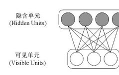
RBM was first proposed and named Harmonium by Paul Smolensky in 1986. As the name suggests, a Restricted Boltzmann Machine is a variant of a Boltzmann Machine. Compared to the usual fully connected graph in a Boltzmann Machine, an RBM is limited to being a bipartite graph, meaning there are undirected connections only between visible units and hidden units, while there are no connections between visible units or between hidden units, as shown in Figure 1. This “restriction” allows for a more efficient training algorithm compared to general BM. It was only after Hinton and his collaborators invented a fast learning algorithm in 2006 that Restricted Boltzmann Machines became widely known.
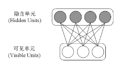 Figure 1 Structure of Restricted Boltzmann Machine Network
DBN‘s training process is typically greedy layer-wise training, where the first RBM is first trained in an unsupervised manner, then its hidden unit layer is used as the visible unit layer of the next RBM, and the next RBM is trained, and so on, stacking multiple RBMs. This layer-wise unsupervised training can be interpreted as a pre-training or weight initialization process, making efficient learning of DBN possible and avoiding the network converging to poor local minima. After layer-wise training is completed, the entire deep network can also undergo further fine-tuning. The objective function for fine-tuning can be unsupervised, as shown in Figure 2 (a), or supervised, as shown in Figure 2 (b). During fine-tuning, the gradient from the top layer not only affects the next layer but also continues to propagate down to all layers below, thus optimizing the network as a whole. The unsupervised deep belief network can abstract input data at different granularities, making one natural application data compression or dimensionality reduction. Another common application is feature extraction, which can effectively characterize the data.
 Figure 2 Structure of Deep Belief Network
2) Deep Autoencoder Network (DAN)
An autoencoder (AE) is an unsupervised artificial neural network aimed at reconstructing inputs, mainly used for learning compressed or over-complete feature representations. Structurally, an autoencoder is a feedforward acyclic network that consists of an input layer, a hidden layer, and an output layer. When the autoencoder contains multiple hidden layers, it forms a deep autoencoder network. The number of nodes in the hidden layer of a deep autoencoder is typically significantly less than that of the input nodes, forming a compressed network structure, so the activation response of the last hidden layer can be regarded as a compressed representation of the input sample. If the number of hidden layer nodes exceeds that of the input layer nodes, the deep autoencoder may learn an identity function, which is meaningless; therefore, additional constraints such as sparsity are usually added to the hidden layer to enable the deep autoencoder network to learn feature representations with specific properties or over-completeness.
The training of deep autoencoders often uses backpropagation methods, such as conjugate gradient descent, steepest descent, etc. However, these methods face optimization challenges for deep autoencoder networks with many layers, such as the gradients diminishing during backpropagation, leading to the inability of the entire network to continue optimizing. The layer-wise pre-training method proposed by Hinton et al. effectively addresses this issue, where two adjacent layers are treated as single-hidden-layer autoencoders for optimization. After layer-wise pre-training, reasonable initial values for all layers’ weights can be obtained, and then the entire network can be fine-tuned to achieve an effective deep autoencoder network. Similar to convolutional neural networks, deep autoencoder networks also easily encounter overfitting issues, and an effective solution is the denoising autoencoder proposed by Vincent et al., which artificially adds noise to the training samples as network inputs, while the outputs remain noise-free samples. This way, the learned network exhibits good robustness to noise, enhancing generalization ability.
In addition to unsupervised feature learning, the autoencoder properties also allow deep autoencoder networks to be used for dynamic texture prediction, signal recovery, denoising, and other purposes. Similar to DBN, to endow the deep autoencoder network with classification and discrimination capabilities, its output layer can be replaced with categories, forming a Softmax layer, and the network weights can be finely adjusted through methods similar to error backpropagation (BP) to obtain a classification or regression network.
3) Deep Convolutional Neural Network (DCNN)
Although the aforementioned DBN and DAN and their corresponding layer-wise, unsupervised pre-training strategies have sounded the bell of the deep learning era and achieved significant progress in problems like speech recognition, the truly killer application success of deep learning comes more from deep convolutional networks (DCNN). The enormous success of DCNN in the field of computer vision has fully ignited the craze of deep learning. Since 2012, based on the deep convolutional neural network LeNet-5 designed by LeCun et al. in 1998, researchers have designed many new deep learning models. The following first briefly introduces LeNet-5 and then discusses several important DCNN models, namely: AlexNet, GoogLeNet, VGGNet, and the recent ResNet.
(1) CNN and LeNet-5
Compared to fully connected networks, the most important feature of the convolutional neural network proposed by LeCun in 1989 is the introduction of convolutional layers, which restrict the non-zero connection weights to local spatiotemporal ranges. It can also be seen as forcing the non-local connection weights in fully connected networks to be zero, extracting local features and effectively retaining spatial positional information. Thus, convolution is essentially a local filtering operation. Compared to fully connected networks, convolution significantly reduces the number of parameters that need to be learned. More importantly, CNN also introduces a weight-sharing strategy, where all neurons in a response map share the same convolutional kernel, further significantly reducing the number of parameters that need to be learned. To extract richer local features, CNN typically sets different sizes and numbers of convolutional kernels at different layers.
Nine years after LeCun first proposed the CNN model in 1989, in 1998, LeCun designed the LeNet-5 network at Bell Labs, which was successfully applied to the handwritten digit recognition system of the United States Postal Service. As shown in Figure 3, the LeNet-5 network has 2 convolutional layers and 2 fully connected layers, where each convolutional layer actually includes three steps: convolution, nonlinear activation function mapping, and downsampling (pooling). The nonlinear activation function (usually using Sigmoid or tanh) endows the network with nonlinear mapping capabilities, while downsampling serves the dual purpose of feature dimensionality reduction and achieving invariance to local changes such as translation. As shown in Figure 3, LeNet-5 uses different numbers of convolutional kernels in the two convolutional layers: the first layer has 6, while the second layer has 16.
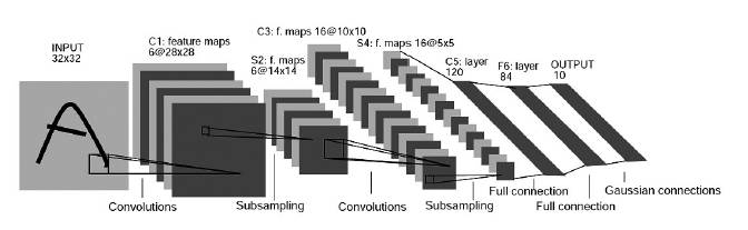 Figure 3 Structure of LeNet-5 Convolutional Network
(2) AlexNet
AlexNet was designed by Hinton’s research group in 2012, participating in that year’s ImageNet competition and achieving the best results in image classification tasks, significantly reducing the error rate of image classification, thus igniting the application craze of deep learning in computer vision. As shown in Figure 4, AlexNet contains 5 convolutional layers and 3 fully connected layers (the last layer is the output layer). Compared to LeNet-5, AlexNet has several important design features: 1) More hidden layers; 2) Introduced a new nonlinear activation function ReLU, replacing the previously commonly used saturation-type nonlinear activation functions (such as Sigmoid, tanh), and practice shows that non-saturated activation functions like ReLU facilitate faster convergence and significantly reduce training time; 3) Adopted Dropout training strategy to prevent overfitting; 4) To solve storage and training speed issues, AlexNet adopted a dual GPU card training structure to process the upper and lower parts of input images separately.
 Figure 4 Structure of AlexNet
(3) GoogLeNet
GoogLeNet is a 22-layer deep convolutional neural network designed by the Google research team in 2014, achieving the best results in the object classification task of the ImageNet competition that year, reducing the Top-5 error rate from 11.7% in 2013 to 6.6%. Compared to AlexNet, GoogLeNet’s core differences lie in: 1) A deeper network structure; 2) A multi-scale convolution structure called Inception. The name Inception is taken from the movie “Inception,” implying a nested convolution structure, as shown in Figure 5, which extracts multi-scale information from the response map through multi-scale convolution operations, enhancing the functionality of the convolution module and improving the network’s nonlinear modeling capabilities.
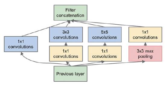 Figure 5 Inception Structure in GoogLeNet
As shown in Figure 6, the entire GoogLeNet stacks multiple Inception structures, resulting in a total network depth of 22 layers. To alleviate the gradient vanishing problem during the training of deep networks, GoogLeNet introduces two auxiliary loss layers in the intermediate layers, i.e., the two Softmax loss layers guided substructures in Figure 5.
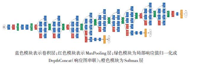 Figure 6 Structure of GoogLeNet
(4) VGG
VGG was designed by Simonyan and Zisserman from the University of Oxford in 2014, achieving first place in the object detection task and second place in the object classification task of the 2014 ImageNet ILSVRC competition. As shown in Figure 7, VGG’s network depth is 16~19 layers, with convolution kernel sizes of 3×3, convolution sampling intervals of 1×1, and Max Pooling intervals of 2×2. As the number of layers increases, the number of convolution kernels increases from 64 to 512. It is worth noting that both VGG and GoogLeNet adopt the practice of consecutive convolutional layers, rather than alternating convolution and pooling layers. VGG and GoogLeNet both indicate that deeper networks are more beneficial for classification, recognition, and other visual tasks.
 Figure 7 Structure of VGG Network
(5) ResNet
ResNet, short for Deep Residual Network, is a DCNN network structure proposed by Kaiming He and others from Microsoft Research at the end of 2015 during the ImageNet competition. Although increasing the depth of the network has been proven to be an effective means to improve performance on practical problems, directly increasing the number of layers leads to a phenomenon known as “degradation”: for example, when the network depth increases from 20 layers to 56 layers on the CIFAR-10 dataset, performance significantly decreases. To address this, ResNet introduces a shortcut structure, as shown in Figure 8. The output of each building block is the sum of the input signal x and the output of the convolutional layer F(x). ResNet eliminates the “degradation” phenomenon during the training of ultra-deep networks, allowing training of networks as deep as 152 layers, achieving championships in two sub-competitions of object recognition and localization, as well as object detection in the ImageNet 2015 competition without relying on external data. The latest improvements to ResNet, namely the identity mapping deep residual network, remove the ReLU operation from the building block, allowing residual terms in different layers of building blocks to be added, with the network depth reaching up to 1001 layers, achieving the current best classification error rate of 4.62% on the CIFAR-10 dataset.
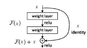 Figure 8 Building Block with Shortcut Structure in ResNet
(6) Fully Convolutional Network (FCN)
For pixel-level classification and regression tasks, such as image segmentation or edge detection, the currently representative deep network model is the Fully Convolutional Network (FCN). Classic DCNNs use fully connected layers after convolutional layers, where individual neurons in the fully connected layer have a receptive field over the entire input image, disrupting the spatial relationships between neurons, thus making them unsuitable for pixel-level visual processing tasks. To address this, as shown in Figure 9, FCN removes the fully connected layers, replacing them with 1×1 convolutional kernels and deconvolutional layers, thereby obtaining outputs with the same size as the input image while maintaining the spatial relationships of the neurons. Furthermore, FCN provides an efficient framework for pixel-level classification and regression tasks through the fusion of multi-scale convolution feature maps across different layers.
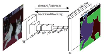 Figure 9 Structure of FCN
4) Recurrent Neural Network (RNN) and Long Short-Term Memory Network (LSTM)
Human understanding of the world is largely based on the information and cognition already present in the mind; for example, when reading an article or watching a movie, context is crucial for understanding the content. Inspired by this, researchers have made structural improvements to traditional neural networks, adding recurrent modules for information retention and transmission, which is the Recurrent Neural Network (RNN). As shown in the left half of Figure 10, the neural network unit A receives input xt, output ht, and the subscript t indicates time. Here, the recurrent structure of module A retains and transmits information in the network from time t to (t+1). The right half of Figure 10 shows the unfolded form of the left diagram’s recurrent structure in chronological order, illustrating the chain-like property that associates RNN closely with (temporal) sequences, making it the most natural network structure for analyzing and processing such data.
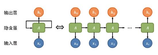 Figure 10 Recurrent Neural Network (RNN) and Its Unfolded Form
Based on the unfolded network structure of RNN, the forward propagation algorithm can sequentially compute input and output in chronological order, then use the backpropagation algorithm (BP) to pass the accumulated residuals from the last time step back to previous steps. This method encounters the “vanishing gradient” problem when dealing with “long-term dependencies,” where the later time nodes’ perception of earlier time nodes diminishes.
The Long Short-Term Memory Network (LSTM) is a special type of RNN proposed by Hochreiter and Schmidhuber in 1997, with many researchers making numerous improvements since then. LSTM introduces new mechanisms to enhance the “memory module,” allowing it to effectively learn long-term dependencies. In traditional RNNs, the recurrent module A is generally composed of a simple activation layer, taking the tanh() function as an example. LSTM retains the chain-like structure of RNN, but the composition of the recurrent module includes 4 neural network layers that interact in a specific way, as shown in Figure 11.
 Figure 11 Composition of LSTM’s Recurrent Module
LSTM’s core idea lies in the state of the unit module, represented as Ct in the figure. The horizontal line from Ct-1 to Ct indicates that the unit state at each time step is transmitted along the entire chain-like structure, with intermediate processes containing only partial linear operations, thus preserving information with minimal loss. Additionally, LSTM can add or remove information from the unit state through a “gates” structure. This operation can be accomplished by a sigmoid neural network layer and pointwise multiplication, outputting values between 0 and 1 to describe the extent of information passage, where 0 indicates complete rejection and 1 indicates complete acceptance. Specifically, LSTM employs three types of gates: forget gate, input gate, and output gate to protect and control the unit state. For the unit module at a certain moment, the first step determines which past information will be removed from the unit state, a decision made by the “forget gate”‘s sigmoid layer (corresponding to the leftmost blue box in Figure 11); the second step determines which new information to store in the unit state: first, the “input gate”‘s sigmoid layer (corresponding to the second left blue box in Figure 11) updates the past information, and then the tanh() activation layer (corresponding to the third left blue box in Figure 11) creates a new candidate state: this requires combining past and new information to determine the new unit state, where the “forget gate” and “input gate” respectively determine the weights (i.e., acceptance levels) of old and new information; the third step determines the unit’s output, which depends on the updated unit state. This is determined by the “output gate” (corresponding to the fourth left blue box in Figure 11) combining input information to determine an acceptance weight. Based on this, the updated unit state passes through an activation layer (corresponding to the rightmost blue box in the figure), multiplied by that weight to produce the output. Through these three steps, the three gates effectively control the frequency and extent of adding and removing information, achieving long-term or short-term memory of information.
In recent years, many sequential problems, such as speech recognition, language modeling, machine translation, image segmentation, and image description generation, have achieved significant results using RNN/LSTM. Additionally, some researchers have designed variants of LSTM based on the actual characteristics of tasks: Gers and Schmidhuber proposed “peephole connections,” where the unit state also serves as input to the gates, and introduced a “coupled forget” mechanism to avoid independent judgment on information removal. A recently popular variant called Gated Recurrent Unit (GRU), proposed by Cho et al., combines the forget and input gates into a single “update gate,” while also merging the unit state and hidden state, resulting in a more simplified and efficient LSTM model.
(Editor: Wang Yuanyuan)
Author Profile:Shan Shiguang, researcher at the Institute of Computing Technology, Chinese Academy of Sciences, with research interests in image processing, computer vision, pattern recognition, and human-computer interaction.
Note:This article was published in the 14th issue of Science and Technology Review in 2016. You are welcome to follow. Some images in this article come from the internet, and copyright matters have not yet been resolved. Authors of the images are welcome to contact us regarding remuneration matters.

Science and Technology Review
Academic Journal of the China Association for Science and Technology
Contact Number: 010-62194182
Long press the QR code to follow