
Editor’s Note
The real-time monitoring of tool wear during machining is of significant importance for reducing equipment downtime and lowering costs caused by tool wear. Traditional tool wear monitoring methods based on signal processing and shallow learning models require manual extraction of lengthy features, which cannot achieve intelligent monitoring. To overcome this inherent limitation, deep learning has been introduced into traditional detection methods. This article summarizes the research status and development trends of intelligent tool wear monitoring methods, specifically analyzing and comparing the advantages and disadvantages of models such as Convolutional Neural Networks (CNN), Recurrent Neural Networks (RNN), and Autoencoders (AE), and summarizes the applications of these models in the field of intelligent tool wear monitoring. Finally, it provides a summary and outlook on the development and challenges of deep learning in the field of intelligent monitoring. In the era of big data, deep learning has enormous advantages and potential in intelligent monitoring.
As one of the most commonly used tools in mechanical manufacturing, tools play an important role in precision machining. The condition of the tool greatly affects the surface quality and machining accuracy of the workpiece during the machining process. Relevant research results indicate that tool wear is the fundamental cause of tool failure, and maintenance costs caused by tool faults account for 15% to 40% of the production cost of goods, while downtime caused by tool faults accounts for about 20% of the total downtime of tools. Therefore, monitoring and predicting the state of tools is of great significance for improving production efficiency and quality and saving costs.
In early studies, traditional machine learning algorithms were primarily used to establish nonlinear mapping relationships between cutting signals and tool wear conditions. Features were extracted from raw signals in the time domain, frequency domain, and time-frequency domain, and then manually selected, such as using Pearson to obtain the correlation coefficient matrix or employing principal component analysis to extract more distinctive features, before inputting the extracted features into machine learning algorithms, mainly including Artificial Neural Networks (ANN), Support Vector Machines (SVM), and Hidden Markov Models (HMM). However, traditional machine learning algorithms have a shallow structural design and cannot extract deeper features. Deep learning, as a data-driven method with strong learning capabilities, has been introduced and applied in various fault diagnosis monitoring, with widely used deep learning models mainly including Convolutional Neural Networks (CNN), Recurrent Neural Networks (RNN), and Autoencoders (AE). Using deep learning for monitoring tool wear can accurately predict the wear state and remaining useful life (RUL) of tools, which is significant for meeting high precision machining requirements and improving automated production rates.
2.1 Forms of Tool Wear
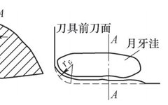
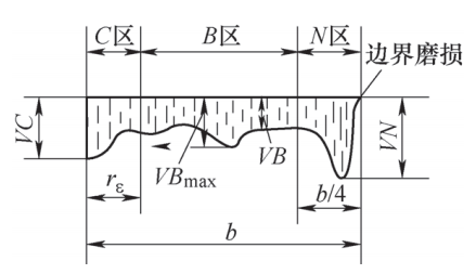
Tool wear is the loss caused by the long-term contact and friction between the tool and the workpiece; under different cutting conditions, the forms of tool wear mainly include flank wear, rake wear, and boundary wear, as shown in Figure 1. Flank wear mainly occurs when the cutting thickness h D and cutting speed v C are large, resulting in a large amount of chips sharply contacting and rubbing against the flank, leading to excessive cutting temperatures and the formation of crescent-shaped notches on the tool, with the wear amount represented by its depth KT. When the cutting thickness h D and cutting speed v C are small, the amount of chips produced is less, and flank wear typically does not occur; however, due to prolonged friction loss, rake wear gradually appears. Rake wear mainly has two forms: wear at the cutting edge and wear at the tool tip. The tip of the tool has poor heat resistance and cooling ability, leading to severe tip wear, with the maximum wear value generally represented by VC . Wear also occurs in the middle position of the cutting edge, but the wear amount here is more uniform, usually represented by VB to indicate its average wear value. Flank wear and rake wear occur when cutting plastic materials and brittle materials, while when cutting harder workpiece materials, deeper groove-like wear occurs, known as boundary wear, with the wear amount represented by the maximum width VN .
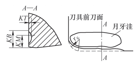
a)Flank Wear
b)Rake Wear and Boundary Wear
Figure 1 Forms of Tool Wear
In many literature studies, due to the fact that rake wear is the ideal failure mechanism for tools, this failure mechanism can be used to identify the wear stage of the tool and predict the remaining useful life. Rake wear can be measured using a microscope, and the values at the wear site are relatively uniform, typically judged by comparing the size of VB to determine whether the tool is currently in a light, moderate, or severe wear stage. A typical tool wear curve is shown in Figure 2, where the identification process of tool wear is essentially the calculation of the wear amount VB. During the cutting process, by monitoring the changes in cutting force, vibration, current, and noise signals, the state of the tool can be monitored; the feature ranges of signals in different states correspond to the respective VB values, and finally, based on the wear amount VB , the wear degree of the tool can be identified. Actual machining processes have proven that timely tool replacement before the wear amount reaches a certain specific value is significant for reducing tool costs and improving machining productivity.
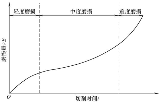
Figure 2 Typical Tool Wear Curve
2.2 Tool Wear Monitoring Methods
According to the different principles of detecting tool wear, tool wear monitoring is mainly divided into direct and indirect methods. The direct method refers to determining the wear state by identifying the geometric shape, surface quality of the cutting edge, or measuring the changes in cutting edge parameters, such as optical methods, radiation methods, and resistance methods; the indirect method monitors not the tool itself, but signals related to the tool, such as cutting force, acoustic emission, vibration, current, and power signals. By obtaining machining tool state information based on the changes in signals during cutting. It is worth noting that although the indirect method has a higher difficulty in model construction and lower accuracy than the direct method, the sensors used are easy to install, can monitor online in real-time, and have lower detection costs. Therefore, the indirect method has been widely used in tool wear monitoring in recent years.
2.3 Traditional Intelligent Tool Wear Monitoring Systems
Traditional intelligent tool wear monitoring systems typically consist of three parts: signal acquisition and processing, feature extraction, and pattern recognition (see Figure 3).
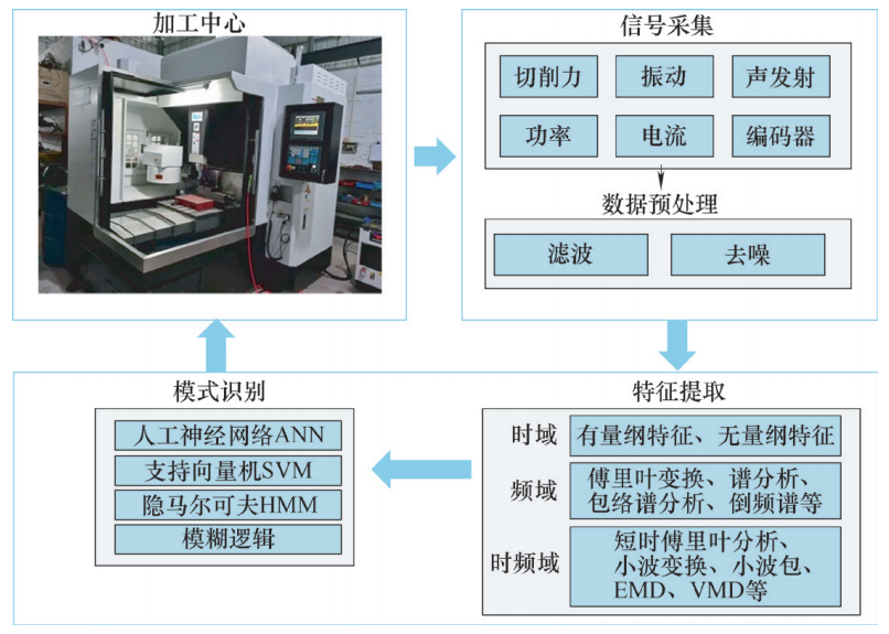
Figure 3 Components of Intelligent Tool Wear State Monitoring System
(1) Signal Acquisition – During the entire tool wear state monitoring process, sensors are the source of signal acquisition for the entire system, and their performance directly affects the accuracy of current monitoring. In current research, cutting force signals, acoustic emission signals, acceleration signals, sound signals, and current signals are typically collected as the basis for judging tool wear. The signal data collected by these sensors have their advantages and disadvantages for identifying tool wear; to address issues such as single sensor signal failure and incomplete collection, multi-sensor fusion technology has gradually emerged as a key to improving the identification rate of monitoring technology.
(2) Feature Extraction – Feature extraction involves extracting useful information from signals that have high sensitivity, reliability, and robustness for identifying tool wear. Feature extraction and selection play a crucial role in tool wear state monitoring, as the extracted feature vector is used for model establishment and testing, which can reduce redundant data, lower dimensions, and improve model identification efficiency and accuracy. Currently, mainstream feature extraction methods include time-domain methods, frequency-domain methods, and time-frequency domain methods.
1) Time-Domain Analysis Method: In time-domain analysis, the processed signal data is transformed into several key feature parameters, including mean, root mean square (RMS), standard deviation, variance, peak value, kurtosis, and margin factor.
2) Frequency-Domain Analysis Method: In frequency-domain analysis, the amplitude spectrum and power spectrum are primarily analyzed, with the most commonly used method being Fourier transform.
3) Time-Frequency Domain Analysis Method: For non-stationary signals, time-frequency domain analysis can jointly locate the time and frequency of the signal. Time-frequency analysis can detect subtle signals without missing useful information, which improves the accuracy of recognition analysis during feature extraction. Currently, commonly used time-frequency analysis methods include wavelet transform (WT), wavelet packet transform (WPT), empirical mode decomposition (EMD), variational mode decomposition (VMD), and various algorithm improvements.
However, not all extracted features can effectively represent the tool wear condition; excessive features can lead to information redundancy, increase training complexity, and reduce model identification accuracy. Therefore, it is necessary to select those features that best represent tool wear state information, reduce data dimensions, and shorten model training time. Currently commonly used feature selection and dimensionality reduction methods include recursive elimination, information entropy gain method, principal component analysis (PCA), and Pearson correlation coefficient method.
(3) Pattern Recognition – The essence of pattern recognition is to use the extracted features as input samples for learning, establishing the corresponding mapping relationship, and completing the identification of the tool wear state based on training. Currently, the construction of monitoring models is mainly divided into two categories: traditional machine learning models and deep learning models. Figure 4 shows the comparison between traditional machine learning and deep learning models.
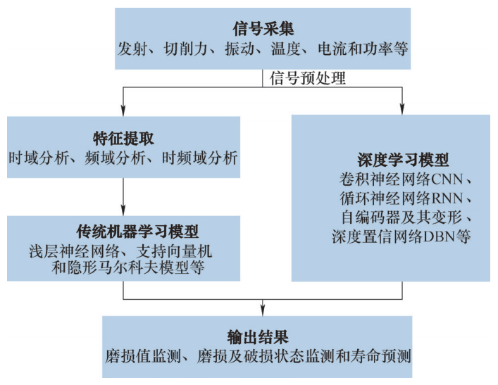
Figure 4 Comparison Between Traditional Machine Learning and Deep Learning Models
Traditional machine learning models require feature extraction and selection from the collected signals, which are then input into the model for learning and recognition. Specific construction methods in traditional models include Artificial Neural Networks (ANN), Support Vector Machines (SVM), and Hidden Markov Models (HMM). RUITAO et al. used wavelet neural networks to predict rake wear, finding that this method can accurately predict the wear degree of tools. CHEN et al. introduced a new method using wavelet packet transform for feature extraction and evaluation during the machining process. ERTUNC et al. proposed a Hidden Markov Model (HMM) for online identification of tool wear based on measurements of cutting force and power signals. AI Changsheng et al. processed cutting sound signals and identified tool wear states using HMM. To address the issue of inaccurate predictions by HMM, extended models of HMM have also been widely applied. KONG D et al. proposed a tool wear estimation model based on Gaussian mixture hidden Markov models and hidden semi-Markov models; He Donglei et al. optimized the algorithms in HMM using genetic algorithms, improving the identification performance of HMM for tool wear states.
Currently, traditional machine learning models are still widely used; however, when the training data volume is too large, the predictive capability of traditional machine learning models is not satisfactory. Deep learning algorithms, with their advantages of adaptive feature extraction, exhibit excellent performance in learning and prediction, achieving higher monitoring accuracy.
Deep learning, as a new method that can learn rules directly from data and extract features, has been extensively researched and introduced into tool wear monitoring. Deep learning models overcome the limitations of cumbersome data preprocessing and manual shallow feature extraction present in traditional machine learning algorithms, making them very suitable for fault classification and recognition prediction, enabling intelligent monitoring of tool wear.
3.1 Tool Wear Monitoring Research Based on Convolutional Neural NetworksCNN
Convolutional Neural Networks (CNN) are deep feedforward neural networks characterized by local connections, weight sharing, etc. The main body of CNN consists of convolutional layers, pooling layers, and fully connected layers. The convolutional layer and pooling layer correspond to feature extraction and dimensionality reduction in traditional signal processing; through continuous alternation and stacking of convolutional layers and pooling layers, CNN can automatically extract local features of the data and establish feature vectors of the data through these local features. After multiple layers of convolution and pooling processing, the data is represented by weighted features from local to global through the fully connected layer, and the results are input to the classifier, which provides the final classification results. The structural framework of CNN is shown in Figure 5.
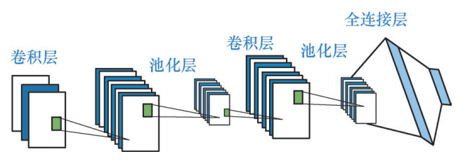
Figure 5 CNN Structure Framework
The scale-invariance and local learning characteristics of CNN lay the foundation for its application in the field of tool wear state monitoring. CAO et al. proposed a highly robust milling tool wear monitoring method based on two-dimensional Convolutional Neural Networks (CNN) and derived wavelet frames (DWF). AMBADEKAR et al. used CNN to monitor the side wear of tools, using images of tools taken periodically by a microscope as input to the CNN model, extracting features and classifying the tool into three wear levels: low, medium, and high. KUMAR et al. designed a deep CNN architecture by selecting appropriate hyperparameters, achieving high classification accuracy for distinguishing between unworn and worn tools in industrial environments.
3.2 Tool Wear Monitoring Research Based on Recurrent Neural NetworksRNN
Recurrent Neural Networks (RNN) are networks with a cyclic structure that include temporal information, performing better than other neural networks when dealing with prediction problems that involve forward and backward dependencies. The entire structure of RNN is divided into three layers: input layer, hidden layer, and output layer. Unlike Multi-Layer Perceptron (MLP), RNN includes a recurrent input from the hidden layer to itself, as shown in Figure 6, which forms a typical feedback neural network structure that has advantages in associative memory and optimization calculations.
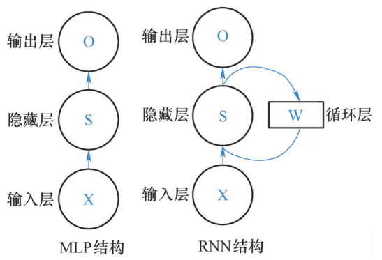
Figure 6 Comparison of Recurrent Neural Networks and MLP
In RNN, the hidden layer units include not only the current input but also the output from the previous time step. The structure of the Recurrent Neural Network is shown in Figure 7, where t-1, t, and t+1 represent three consecutive input moments; x represents input; y is the corresponding output; S is the hidden state; U, V, and W correspond to the weights from input layer to hidden layer, hidden layer to hidden layer, and hidden layer to output layer, respectively.
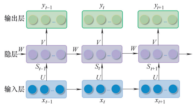
Figure 7 Structure of Recurrent Neural Network
Tool wear is a gradual process that changes with machining time, and mining temporal features is important for predicting tool wear at various moments. For temporal signals during the machining process, under mixed faults and strong noise, YAO et al. proposed a deep transfer reinforcement learning (DTRL) network based on Long Short-Term Memory (LSTM) networks, extracting local features from continuous sensor data to track tool states and dynamically adjusting the size of the trained network by controlling the length of the time series. LIU et al. proposed a TWM model based on parallel residual stacked bidirectional LSTM networks. The proposed network can simultaneously extract spatio-temporal correlation features from the original signals, achieving a multi-feature fusion structure through parallel residual networks, resulting in high prediction accuracy. AN et al. combined CNN with stacked bidirectional and unidirectional LSTM networks (CNN-SBULSTM) for sequential data processing in tool RUL prediction tasks, obtaining deeper and more abstract features without the need for feature engineering and difficult-to-obtain high-quality expert knowledge, with an average prediction accuracy of up to 90%. LSTM networks are highly applicable in tool wear monitoring and prediction.
3.3 Tool Wear Monitoring Research Based on AutoencodersAE
Autoencoders (AE) are unsupervised deep learning networks used for data dimensionality reduction and feature extraction, with the architecture shown in Figure 8, including input layer, hidden layer, and output layer. The original data is mapped to the hidden layer through weight connections, and the activation values of the hidden layer are mapped to the output layer for data reconstruction, minimizing reconstruction errors and fine-tuning weights to generate accurate data representations. The main computational formulas for Autoencoders are as follows:
Decoding Process:
h = Sg(Wx + b) (1)
Encoding Process:
z = Sf(W’h + b’) (2)
In the formula, C1 is the cost function of the AE; β is the sparse penalty coefficient; r is a sparse constant; x = [x1, x2, …, xm] is a feature vector of unlabeled input samples; z = [z1, z2, …, zm] and h = [h1, h2, …, hm]; Sg and Sf are the activation functions for the hidden layer and output layer, usually using Sigmoid (Sigm) or Rectified Linear Unit (ReLU) as activation functions; W and W’ are weights; b and b’ are biases.
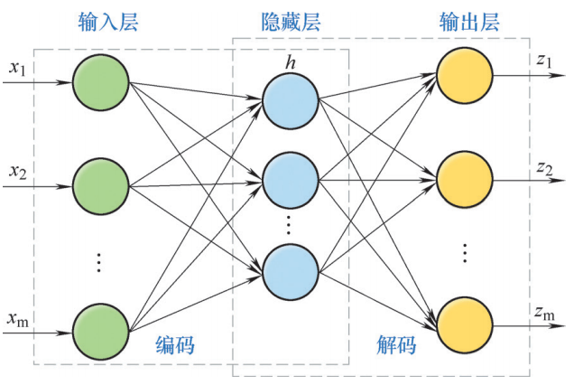
Figure 8 AE Model Architecture
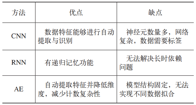
The comparison of intelligent monitoring methods for tool wear based on deep learning is shown in Table 1.
Table 1 Comparison of Intelligent Tool Wear Monitoring Methods Based on Deep Learning
Deep learning, as a new method for intelligent state monitoring, has good characteristics in autonomously learning data feature extraction compared to traditional signal processing and shallow machine learning models. Deep learning, with its adaptive feature extraction approach, eliminates the need for manual feature extraction and selection, and with its ability to approximate nonlinear functions, avoids the issues of missed features during manual extraction, making the extracted feature information more sensitive and robust. Through a layer-by-layer learning approach, it is easier to learn useful deep information from the original data, improving monitoring recognition accuracy.
As the influence of Industry 4.0 on traditional mechanical manufacturing continues to grow, it is expected that deep learning will have further research and development in the field of intelligent monitoring.
-End-
☞ Source: Metal Processing ☞ Media Cooperation: 010-88379798 ext. 520 ☞ The only submission website for Metal Processing Magazine: http://tougao.mw1950.cn/

Submission Guidelines
“Metal Processing (Cold Processing)” magazine submission scope: processing technology schemes for metal components in aerospace, automotive, rail transportation, engineering machinery, molds, ships, medical devices, and energy industries, design/manufacturing schemes for fixtures, tool design/processing schemes, intelligent manufacturing (programming design, optimization) schemes, as well as maintenance and modification schemes for mechanical equipment or tools.
Please contact for submissions: Han Jingchun, 010-88379790-518, 18501077977 (same as WeChat)
Submission Guidelines:Please click“Metal Processing (Cold Processing)” magazine submission specifications