Deep Learning Model Training and Debugging: Efficient Tools and Concepts (Part 1)

“IT has something to talk about” is a professional IT information and service platform under the Machinery Industry Press, dedicated to helping readers master more professional and practical knowledge and skills in the broad IT field, quickly enhancing their workplace competitiveness. Click the blue WeChat name to quickly follow us!

PART1: Dataset

In PyTorch, a dataset is represented by a regular Python class that inherits from the Dataset class. You can think of it as a list of tuples, where each tuple corresponds to a point (feature, label).

The most basic methods it needs to implement are:

• __init__(self): It takes any parameters needed to construct the list of tuples—it could be the name of a CSV file to be loaded and processed; it could also be two tensors, one for features and the other for labels; or anything else, depending on the current task.

There is no need to load the entire dataset in the constructor (__init__). If your dataset is large (like thousands of image files), loading it all at once will not save memory; it is recommended to load them on demand (whenever __get_item__ is called).

• __get_item__(self,index): It allows indexing into the dataset so that it can work like a list (dataset[i])—it must return the tuple (feature, label) corresponding to the requested data point. It can return the corresponding slice of a pre-loaded dataset or load them on demand as mentioned above.

• __len__(self): It should simply return the size of the entire dataset, so that whenever it is sampled, its index is limited to the actual size.

Build a simple custom dataset that requires two tensors as parameters: one for features and one for labels. For any given index, the dataset class will return the corresponding slice of each tensor. The code is as follows:

class CustomDataset(Dataset):    def __init__(self, x_tensor, y_tensor):        self.x = x_tensor        self.y = y_tensor
    def __getitem__(self, index):        return (self.x[index], self.y[index])
    def __len__(self):        return len(self.x)
# Wait, is this a CPU tensor? Why? Where is .to(device)?
x_train_tensor = torch.from_numpy(x_train).float()
y_train_tensor = torch.from_numpy(y_train).float()
train_data = CustomDataset(x_train_tensor, y_train_tensor)
print(train_data[0])

Output

(tensor([0.7713]), tensor([2.4745]))

Deep Learning Model Training and Debugging: Efficient Tools and Concepts (Part 1)

Did you notice that the training tensors were built using Numpy arrays but were not sent to the device? So, they are now CPU tensors! Why? We do not want the entire training data to be loaded into GPU tensors because it occupies our precious GPU memory space.

TensorDataset

Again, you might wonder, “Why wrap several tensors in a class?” Once again, you are right… If a dataset is just a few tensors, you can use PyTorch’s TensorDataset class, which works almost the same as the custom dataset above.

So now, the mature custom dataset class may seem a bit contrived, but we will reuse this structure in later chapters. For now, enjoy the simplicity of the TensorDataset class.

train_data = TensorDataset(x_train_tensor, y_train_tensor)
print(train_data[0])

Output

(tensor([0.7713]), tensor([2.4745]))

Great, but then again, why build a dataset? We do this because we want to use…

PART2: DataLoader

So far, we have been using the entire training data at each training step. It has been batch gradient descent. Of course, this is fine for very small datasets, but if you want to take this seriously, you must use mini-batch gradient descent. Thus, mini-batches are needed. Therefore, the dataset needs to be split accordingly.

So use the DataLoader class from PyTorch to do this. Tell it which dataset to use (the one we just built in the previous section), the desired mini-batch size, and whether you want to shuffle it.

Important Note: In most cases, you should set shuffle=True for your training set to improve the performance of gradient descent. However, there are some exceptions, such as time series problems, where shuffling can actually lead to data leakage.

So I always ask myself: “Do I have a reason not to shuffle the data??”“What about the validation and test sets?”There is no need to shuffle them because there is no gradient calculation done with them.

The functionality of DataLoader goes far beyond what meets the eye… For instance, it can also be used with samplers to obtain mini-batches that compensate for imbalanced classes. There is too much to handle right now, but we will get to it eventually.

Our loader will behave like an iterator, so we can loop through it and get different mini-batches each time.

“How do I choose the mini-batch size?”

For mini-batch sizes, powers of 2 are often used, such as 16, 32, 64, or 128, with 32 seeming to be the choice of most, including Yann LeCun.

Some more complex models might use larger sizes, although the size is usually limited by hardware (i.e., the actual number of data points that can be loaded into memory).

In our example, there are only 80 training points, so I chose a mini-batch size of 16 to conveniently split the training set into 5 mini-batches.

train_loader = DataLoader(dataset=train_data, batch_size=16, shuffle=True)

To retrieve a mini-batch, you can simply run the following command—it will return a list containing two tensors, one for features and the other for labels:

next(iter(train_loader))

Output:

[tensor([[0.1196],[0.1395],...[0.8155],[0.5979]]), tensor([[1.3214],[1.3051],...[2.6606],[2.0407]])]

“Why not use a list?”

If you call list(train_loader), you will get a list; the result is a list containing 5 elements, which are all 5 mini-batches. Then you can use the first element of that list to get a single mini-batch, as shown above. This defeats the purpose of using the DataLoader iterable object, which is to iterate one element (in this case, a mini-batch) at a time.

To learn more, check out RealPython’s materials on iterables and iterators. How does this change the code so far? Let’s take a look!

First, we need to add the Dataset and DataLoader elements to the data preparation section of the code. Also, note that the tensors have not yet been sent to the device. The code is as follows:

Define—Data Preparation V1

%%writefile data_preparation/v1.py
# Data is in Numpy arrays
# But needs to be converted to PyTorch tensors
x_train_tensor = torch.from_numpy(x_train).float()
y_train_tensor = torch.from_numpy(y_train).float()
# Build Dataset
train_data = TensorDataset(x_train_tensor, y_train_tensor)  ①
# Build DataLoader
train_loader = DataLoader(dataset=train_data, batch_size=16, shuffle=True)  ②

① Build a tensor dataset.

② Build a data loader that generates mini-batches of size 16.

Run—Data Preparation V1

%run -i data_preparation/v1.py

Next, we need to merge the mini-batch gradient descent logic into the model training part of the code. But we need to run the model configuration first.

Run—Model Configuration V1

%run -i model_configuration/v1.py

Define—Model Training V2

%%writefile model_training/v2.py
# Define the number of epochs
n_epochs = 1000
losses = []
# For each epoch…
for epoch in range(n_epochs):    # Inner loop    mini_batch_losses = []  ④    for x_batch, y_batch in train_loader:   ①        # The dataset “exists” in CPU, so do the mini-batches        # Therefore, these mini-batches need to be sent to the device        x_batch = x_batch.to(device)   ②        y_batch = y_batch.to(device)   ②
        # Perform a training step        # and return the corresponding loss for this mini-batch        mini_batch_loss = train_step(x_batch, y_batch)   ③        mini_batch_losses.append(mini_batch_loss)   ④
    # Calculate the average loss of all mini-batches—this is the loss for the epoch    loss = np.mean(mini_batch_losses)   ⑤
    losses.append(loss)

① Inner loop for mini-batch.

② Send a mini-batch to the device.

③ Perform a training step.

④ Track the loss within each mini-batch.

⑤ Average the mini-batch losses to get the epoch loss.

Run—Model Training V2

%run -i model_training/v2.py

“Wow! What happened here?!”

It seems a lot has changed… Let’s take a close look step by step:

• An inner loop was added to handle the mini-batches generated by the DataLoader (line 12).

• Only one mini-batch was sent to the device instead of sending the entire training set (lines 16 and 17).

For larger datasets, loading data on demand in the __get_item__ method of the Dataset (into CPU tensors), and then sending all data points belonging to the same mini-batch immediately to your GPU (device) is a great way to utilize GPU memory.

Additionally, if you have multiple GPUs to train your model, it is better to keep your dataset “device-independent” and assign batches to different GPUs during training.

• A train_step was performed on one mini-batch (line 21) and the corresponding loss was appended to a list (line 22).

• After iterating through all mini-batches, at the end of an epoch, the total loss for that epoch was calculated, which is the average loss of all mini-batches, and the result was appended to a list (lines 25 and 27).

After two updates, the current development state is:

• Data Preparation V1.

• Model Configuration V1.

• Model Training V2.

Not so bad, right? So, it’s time to check if the code still works:

# Check the model parameters
print(model.state_dict())

Output

OrderedDict([('0.weight', tensor([[1.9684]], device='cuda:0')),            ('0.bias', tensor([1.0235], device='cuda:0'))])

Did you get slightly different values? Try running the entire pipeline again:

Complete Pipeline

%run -i data_preparation/v1.py
%run -i model_configuration/v1.py
%run -i model_training/v2.py

Since the DataLoader samples randomly, executing other code between the last two steps of the pipeline may interfere with the reproducibility of the results.

Anyway, as long as your results differ from my weights and biases by less than 0.01, your code is working fine.

Did you notice that the training time is longer now? Can you guess why?

The answer: The training time is longer now because each epoch executes the inner loop five times (in our example, this is because we use a mini-batch size of 16 and there are a total of 80 training data points, so the inner loop executes 80 / 16 = 5 times). Therefore, the total number of train_step calls is now 5000! No wonder it takes longer!

Mini-batch Inner Loop

full batch gradient descent again. So it makes sense to organize a piece of code that will be reused into its own function (mini-batch inner loop)!

The inner loop depends on the following 3 elements:

• The device to which the data is sent.

• The data loader from which mini-batches are extracted.

• A step function that returns the corresponding loss.

Taking these elements as inputs and using them to execute the inner loop will yield the following function:

Helper Function 2

def mini_batch(device, data_loader, step):    mini_batch_losses = []    for x_batch, y_batch in data_loader:        x_batch = x_batch.to(device)        y_batch = y_batch.to(device)
        mini_batch_loss = step(x_batch, y_batch)        mini_batch_losses.append(mini_batch_loss)
    loss = np.mean(mini_batch_losses)    return loss

In the previous section, we realized that due to the mini-batch inner loop, we performed over five times the updates (train_step function) for each epoch. Previously, 1000 epochs meant 1000 updates. Now, only 200 epochs are needed to perform the same 1,000 updates.

How does the training loop look now? Very streamlined!

Run—Data Preparation V1, Model Configuration V1

%run -i data_preparation/v1.py
%run -i model_configuration/v1.py

Define—Model Training V3

%%writefile model_training/v3.py
# Define the number of epochs
n_epochs = 200
losses = []
for epoch in range(n_epochs):    # Inner loop    loss = mini_batch(device, train_loader, train_step)   ①    losses.append(loss)

① Perform mini-batch gradient descent.

Run—Model Training V3

%run -i model_training/v3.py

After updating the model training part, the current development state is:

• Data Preparation V1

• Model Configuration V1

• Model Training V3.

Check the model state:

# Check the model parameters
print(model.state_dict())

Output

OrderedDict([('0.weight', tensor([[1.9687]], device='cuda:0')),            ('0.bias', tensor([1.0236], device='cuda:0'))])

So far, we have only focused on the training data. We can do the same for the validation data, using the split performed at the beginning of this book… or we can use random_split instead.

Random Split

The random_split() method in PyTorch is a simple and mature way to perform train-validation splits.

So far, we have been using x_train_tensor and y_train_tensor built based on the original split from Numpy to construct the training dataset. Now, we will use the complete data from Numpy (and ), first to build a PyTorch dataset, and then use random_split() to split the data.

So for each data subset, a corresponding DataLoader is built, so the code is as follows:

Define—Data Preparation V2

%%writefile data_preparation/v2.py
torch.manual_seed(13)
# Build tensors from numpy arrays before splitting
x_tensor = torch.from_numpy(x).float()  ①
y_tensor = torch.from_numpy(y).float()  ①
# Build a dataset containing all data points
dataset = TensorDataset(x_tensor, y_tensor)
# Perform the split
ratio = .8
n_total = len(dataset)
n_train = int(n_total * ratio)
n_val = n_total - n_train
train_data, val_data = random_split(dataset, [n_train, n_val])   ②
# Build loaders for each set
train_loader = DataLoader(dataset=train_data, batch_size=16, shuffle=True)
val_loader = DataLoader(dataset=val_data, batch_size=16)   ③

① Generate tensors from the complete dataset (before splitting).

② Perform train-validation split in PyTorch.

③ Create a data loader for the validation set.

Run—Data Preparation V2

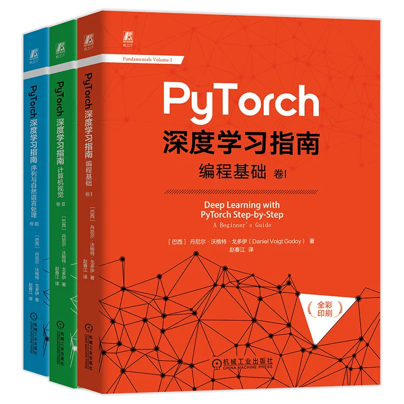
%run -i data_preparation/v2.py

Now that we have a data loader for the validation set, let’s use it for…

The above content is excerpted from PyTorch Deep Learning Guide: Programming Basics Volume I

Author: [Brazil] Daniel Voigt Godoy

In this section, we explained Dataset and DataLoader, and in the next section, we will continue to present content on evaluation and TensorBoard.

PART3: Recommended Reading

▊《PyTorch Deep Learning Guide》

[Brazil] Daniel Voigt Godoy, translated by Zhao Chunjiang

“The PyTorch Deep Learning Guide” series systematically explains important concepts, algorithms, and models related to deep learning, focusing on how PyTorch implements these algorithms and models. The book is divided into three volumes: Volume I Programming Basics, Volume II Computer Vision, Volume III Sequences and Natural Language Processing.

Written by: Ji Xu

Editor: Zhang Shuqian

Reviewer: Cao Xinyu

Leave a Comment Cancel reply