Deep Feedforward Networks

Introduction

This series of articles serves as notes on the book “Deep Learning”. It is recommended to refer to the original book for a better reading experience. Starting from this article, we will continue to learn the second part of the book, transitioning from the foundational knowledge of deep learning introduced in the first part to constructing deep networks, which is the application and enhancement of theory.

Deep Feedforward Networks

Also known as Multilayer Perceptrons or Feedforward Neural Networks, this is a typical deep learning model. This model is a forward mapping model, where the initial input is mapped to the output y through function f, and there is no feedback from the output to the model itself (the type with feedback is called a recurrent neural network). Here, the concept of a network is a directed acyclic graph, the simplest being a chain connection, where input x passes through f1, then f2, then f3, and finally outputs to result y. The concept of layers is introduced, where f2 is one layer, and f3 is the output layer. The training data provides x and y but does not define the inputs and outputs of the intermediate layers, hence the intermediate layers are also called hidden layers.

Linear models are divided into logistic regression (for classification problems) and linear regression (for continuous value prediction problems), which can fit efficiently and reliably. However, the limitation is that their capability is confined to linear functions and cannot understand the interactions between input variables. Therefore, we consider applying a nonlinear transformation φ(x) to the input x, followed by a linear function acting on φ(x). The questions involved here are how to choose φ(x):

1. A general φ with sufficiently high dimensions can fit the input and output well, but the problem is that generalization is often poor.

2. Manually designed φ, where experts design algorithms and manually code φ, but this is algorithm design targeted at specific problems and is difficult to transfer.

3. Learning φ, where φ(x;θ) will be trained with parameter θ, and can help generalization by using a wide range of function families or human coding to achieve the above two scenarios.

Learning the XOR Function

The meaning of XOR is: x1 and x2 are the same, output 0; if different, output 1. We set the cost function as:

Solving gives: w=0, b=1/2, which is obviously incorrect. Why is this the case? When x1=0, the model output increases with x2, and when x1=1, the model output decreases with x2. How could a linear model achieve this? Hence, we obtained an incorrect result.

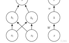
To solve this problem, we introduce a hidden layer to form the feedforward neural network:

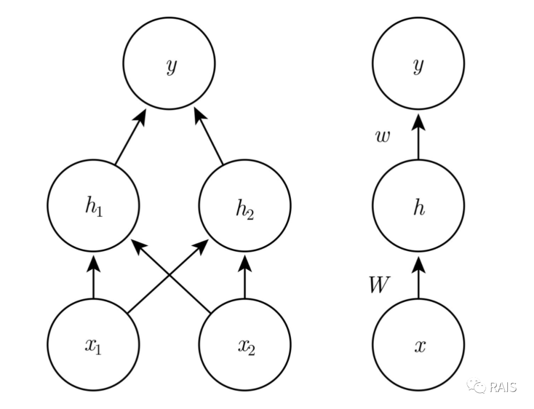
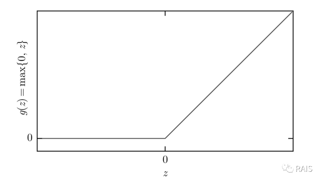
Here we need to consider what kind of function h should be. If it is a linear function, substituting into y would yield a linear function result again. From previous analysis, we know this cannot meet the requirements, so h must be a nonlinear function. Here we use an activation function, the Rectified Linear Unit (ReLU): g(z)=max{0, z}.

Thus the network is:

We can then calculate the result:

At this point, we have completed the construction of the XOR function based on the deep learning model.

Conclusion

Here, we have constructed a very simple deep feedforward network. Understanding the network model is a mathematical mapping or function representation; there is no judgment like the same being 0 and different being 1, but rather a matrix operation, which is a transformation of thinking. Computers represent a solidified form of mathematics, which is particularly evident here. In the next article, we will discuss gradient learning from a new perspective.