The previous article on AIGC basics, from VAE to DDPM principles and code details, has introduced the basic principles of image generation based on diffusion models in a relatively detailed manner. However, in the real industry, to achieve controllable image generation, there are still many practical problems that need to be solved, such as the following:
1. How are the control conditions injected into the model to control the generated image?
2. How to generate high-definition images with sufficiently realistic details?
3. How to reduce parameters and computational load in model design?
4. Besides text, how to use other forms of conditional control?
With these typical questions in mind, this article attempts to share several of the most representative models for text-controlled image generation: OpenAI’s DALL-E-2【1】, Google’s ImaGen【2】, Stability.AI’s Latent Stable Diffusion【3】, and Stanford’s latest ControlNet【4】. These models all utilize the diffusion technology introduced above. Since these generative models are composed of multiple typical technical modules rather than a single model, when sharing the above models, I will also briefly introduce several other typical models involved in these models, such as CLIP【5】, T5【6】, and the diffusion-based super-resolution model.
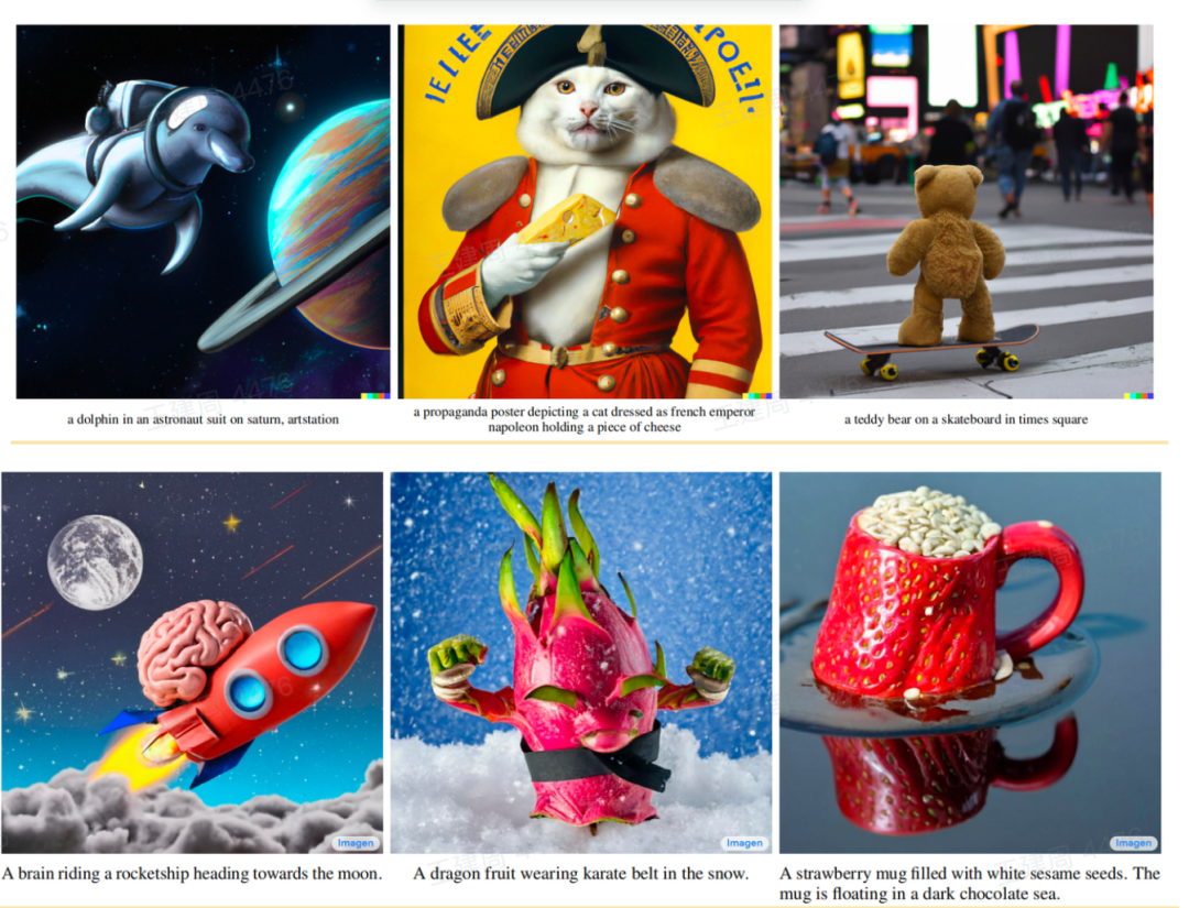
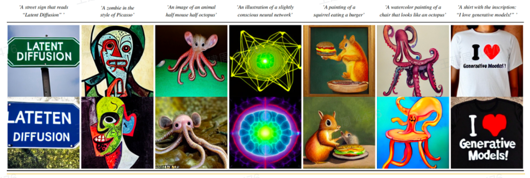
Below are the images generated by DALL-E-2, ImaGen, and Stable Diffusion.
2. DALL-E-2
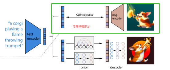
DALL-E-2 essentially belongs to the classifier-free diffusion model mentioned above, where the condition is the input text. The overall architecture of the model is shown in the figure below, and the green box part (which belongs to CLIP) can be ignored for now.
The model is divided into four main parts (one part is not shown in the figure, belonging to the non-essential part of text-image generation), and the entire generation process is executed sequentially through these four parts.
1. Text encoder: Encodes the input text into a vector.
2. Prior module: Converts the text vector into an image vector, which serves as the control condition for the decoder.
3. Decoder: Decodes the image vector into an image using the diffusion model.
4. SR super-resolution module: Enhances the image generated in step 3 to a higher resolution image using super-resolution technology.
These four parts are trained separately in DALL-E-2 rather than jointly in an end-to-end manner. Next, I will detail the content of these four parts (since the original paper of DALL-E-2 lacks many details, some subjective guesses will be made).
1. Text Encoder
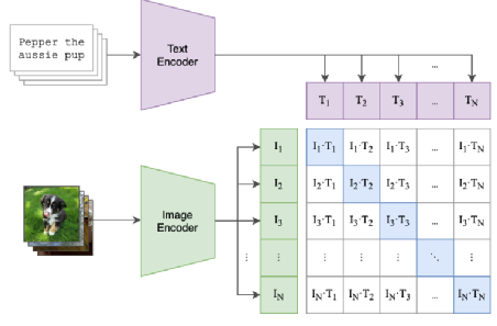
The purpose of the text encoder is to convert text into a mathematical representation vector, hoping to capture the semantic meaning of the text in this process while linking the semantic meaning of the text describing the image with the semantic meaning of the image. In the DALL-E-2 model, the CLIP model is used. The CLIP model also comes from OpenAI and has a straightforward starting point: linking images and their descriptive texts through contrastive learning, hoping that the representation vector of an image and the representation vector of this image’s descriptive text
 are close, while hoping
 to be sufficiently far from other image text vectors
 as shown in the figure below.
The pseudo-code implementation is as follows, using InfoNCE as the most common loss for contrastive learning:
as shown in the figure below.
The pseudo-code implementation is as follows, using InfoNCE as the most common loss for contrastive learning:
def clip_training(imgs, texts): # The batch size of imgs and texts should be as large as possible; the larger the contrastive learning batch size, the better the effect. # The image encoder and text encoder encode images and texts into comparably sized embeddings. img_embedding = img_encoder(imgs) txt_embedding = text_encoder(texts) norm_img_embedding = tf.nn.l2_normalize(img_embedding, -1) norm_txt_embedding = tf.nn.l2_normalize(txt_embedding, -1) logits = tf.matmul(norm_txt_embedding,norm_img_embedding,transpose_b=True) batch_size = tf.range(tf.shape(imgs)[0]) label = tf.range(batch_size) # Simplified implementation of infonce, considering the diagonal part of the similarity matrix as label=1, other parts as label=0. loss1 = tf.keras.losses.sparse_categorical_crossentropy( label, logits, from_logits=True ) # Non-diagonal parts swap, implementing t and i, i and t calculations. loss2 = tf.keras.losses.sparse_categorical_crossentropy( label, tf.transpose(logits), from_logits=True ) return (loss1+loss2)/2.0
The CLIP model is trained on 4 billion image-text pairs, which can effectively link text semantics with image semantics. By constructing prompts in classification tasks, it can surpass SOTA image classification models on some abstract images.
Once CLIP is trained, it is frozen, and the img_encoder and text_encoder trained within CLIP will be used later.
2. Prior Module
For images x and descriptions y (control conditions) in the training set, as well as the image and text feature vectors zi,zt obtained through CLIP, the likelihood model we expect is p(x|y), which can be derived as follows:
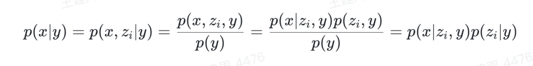
This indicates that introducing zi obtained from y makes the model equivalent.
How to obtain zi from y? In the paper, the authors tried autoregressive and diffusion models, and after comparing effectiveness and efficiency, they ultimately used the diffusion model. The input to this diffusion model consists of the following:
1. y, which is the description of the image.
2. zt, which is the vector obtained from the image description through the CLIP text encoder.
3. t, which is the time step in the diffusion model.
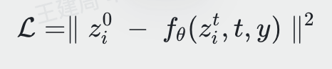
In common cases, the diffusion model predicts noise very well, but in the Prior module of DALL-E-2, the authors found that directly predicting zi yields better results. The derivation of the formula is as follows; from formula 88, we can obtain:

The logic of predicting noise is as follows: Given xt, we can design the following objective (assuming ).
).
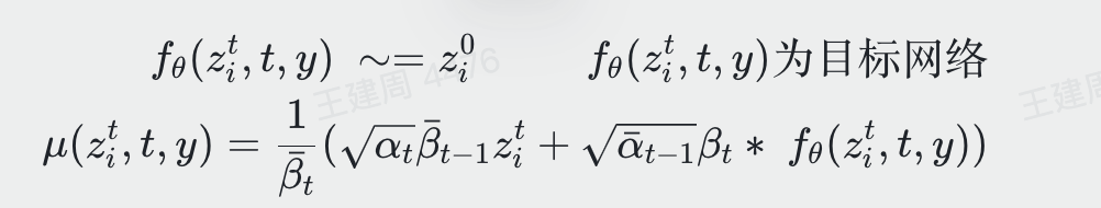
After deriving it similarly to the above formula 130, the final loss becomes as follows:
When the Prior finally outputs Zi, there is an additional operation: the Prior generates two Zi, and selects the one most similar to Zt as the control condition for the decoder. Note that the Prior module is not mandatory; as seen in the model architecture diagram, we can also directly use the text vector Zt. The paper found that doing so yields suboptimal image generation results; additionally, to accelerate the diffusion generation, the DDIM jump sampling method was used to reduce the number of sampling steps.
3. Decoder Module
The Decoder module is the classifier-free diffusion model mentioned above, where the condition is the output Zi from the Prior module, and I will not elaborate further here.
4. SR Super-resolution Module
As seen above, the diffusion model calculates on the input image size and requires a very large number of calculations, so it is very slow on large images. To speed up the generation process, smaller images are generally generated first, and then restored to larger images using super-resolution. Currently, the SOTA SR models also mostly use diffusion technology. DALL-E-2 uses two diffusion-based super-resolution models, first restoring the generated 64×64 image to 256×256, and then to 1024×1024.
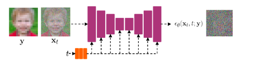
The diffusion-based SR also uses classifier-free diffusion, where the low-resolution image is the control condition y, and the high-resolution image is x, which is our final target to be generated. Thus, the model becomes p(x|y), and each training step is shown in the figure below:
3. ImaGen
ImaGen comes from Google Research and essentially also belongs to the classifier-free diffusion model. The overall model architecture diagram is as follows:
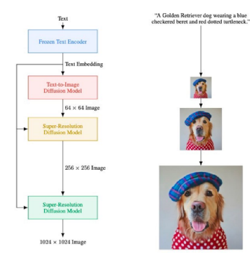
It is very similar to DALL-E-2, with the only major module missing being the Prior module. It is mainly divided into the following parts:
1. Text encoder: Outputs text embedding.
2. Text to Image Diffusion Model: This serves the same purpose as the Decoder of DALL-E-2, using classifier-free diffusion to generate images, where the control condition y is the text embedding from the first step.
3. Two cascaded super-resolution image modules. Unlike DALL-E-2’s super-resolution module, ImaGen’s super-resolution module takes both the low-resolution image and the text embedding as input.
Below I will briefly introduce these modules.
In ImaGen, the text encoder used is T5-XXL, a model pre-trained purely on natural language. Because the scale and diversity of training data for texts far exceed that of image descriptions in image-text pairs, its understanding of text semantics is better than that of the CLIP Text encoder. However, it lacks cross-modal training, so it lacks alignment between text semantics and image semantics. However, from the final generated image results, this does not detract from its performance compared to DALL-E-2. Thus, in text-to-image generation tasks, as long as the pre-trained text encoder can effectively extract text semantics, it does not matter whether this feature aligns with image features.
This paper also finds that if a pre-trained text encoding model is used, the stronger the model, the better the final generated image quality (this is easy to understand; if two semantically different texts cannot be distinguished by the text encoder, the generated images must also be visually indistinguishable). For instance, the subjective scoring of generated images improves when the text encoder is upgraded from T5-small to T5-XXL. Here is a brief introduction to T5.
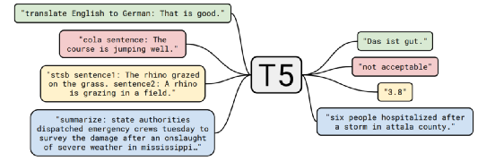
T5 is a unified modeling approach for natural language tasks (previously, tasks like NER were modeled separately; classification required a classification head; and translation was a sequence-to-sequence task) through sequence-to-sequence generation. The model’s input is: task description (prompt) + input text, and it decodes the answers step by step through autoregression, as illustrated in the figure below (the left side is model input, and the part before the colon is the prompt; the right side is the model’s generated output).
This method not only unifies the modeling of different natural language tasks but also has the advantage of unifying self-supervised pre-training and final target tasks, thus enhancing zero-shot performance.
The generative model architecture has the following three types (currently, every layer of the model basically uses transformers).
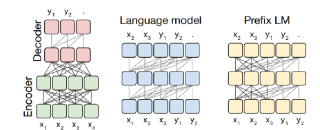
1. On the far left, encoder-decoder: the encoder can see all the text information to obtain the encoded vector; the decoder generates in an autoregressive manner, so during training, it uses a causal mask to ensure the decoder can only see the current time step’s preceding text information and the encoder’s output vector.
2. The middle decoder: similar to the left decoder, but lacks the output vector from the encoder.
3. PrefixLM: a hybrid of the first two, where some layers of the model can see all the text, while some can only see the preceding text information at the current time step.
Ultimately, T5 chose the first type (the GPT series models are all of the second type, which perform better on generative tasks).
2. Text to Image Diffusion Model
The image generation module of ImaGen uses classifier-free diffusion model to generate images, where the control condition y is the text embedding from the first step; I will not elaborate further here.
However, there is a detail worth learning in this step: in the diffusion model, the input image is normalized to the range [-1,1]. However, during the multi-step diffusion process, the model’s output features tend to exceed this range, making training difficult and causing inconsistencies between training and final sampling generation. Therefore, ImaGen addressed this issue using truncation processing, attempting both threshold and ratio truncation:
1. Threshold truncation: Simply scale any model output greater than 1 to 1 and any output less than -1 to -1, thus ensuring the model’s output remains within [-1,1].
2. Ratio truncation: Statistically analyze the model’s output pixel values, select a determined value s, and ensure that the pixels within the range [-s,s] meet a certain ratio. Pixel values exceeding the threshold of [-s,s] are truncated to -s and s, and the truncated values are normalized to [-1,1] by dividing by s.
After effect analysis, it was found that ratio truncation yields better results. This is easy to understand; as t increases, the pixels of the model’s output that fall outside the static threshold of [-1,1] increase, and directly converting these pixels to -1 and 1 leads to significant detail loss.
3. Cascaded Super-resolution Module
The output image size from the Text to Image Diffusion Model is 64×64. ImaGen employs two levels of super-resolution modules to upscale the image to 1024×1024. The image generation module uses super-resolution modules based on classifier-free diffusion model. Unlike DALL-E-2’s super-resolution module, ImaGen’s super-resolution module uses not only the low-resolution image but also the encoded vector from the text encoder as input.
The paper mentions the use of cross-attention to integrate the text vector, which I personally speculate is consistent with Stable Diffusion, which will be discussed later.
4. Latent Stable Diffusion Model
The Latent Stable Diffusion Model (LDM) was developed by Stability.AI and is fully open-sourced, with many entrepreneurial products like Lensa already built on this open-source pre-trained model.

LDM essentially also employs the classifier-free diffusion model, which has two notable characteristics:
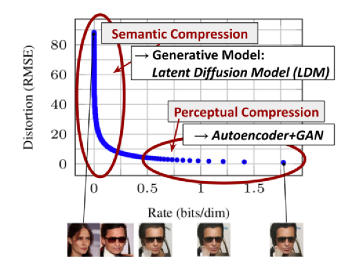
1. Compared to DALL-E-2 and ImaGen, which perform diffusion directly on images, LDM performs diffusion in a latent space learned from a model similar to VAE or VQVAE. Since the number of features in the latent representation is much smaller than the original image pixels, this greatly reduces the computational load during the multi-step diffusion process, allowing the model to run on low-power devices. Of course, this approach also requires careful consideration, as most pixel points in an image are redundant for semantic information, while our controllable diffusion model primarily aims to control the image semantics. The image below shows how the pixel-level semantic information can be greatly compressed.
 2. Compared to other classifier-free diffusion models, the condition is integrated into the model through simple addition or concatenation. LDM employs cross-attention for fusion, allowing the model to better capture the correlation between different types of control conditions y and images.
The entire model architecture is shown in the figure below:
2. Compared to other classifier-free diffusion models, the condition is integrated into the model through simple addition or concatenation. LDM employs cross-attention for fusion, allowing the model to better capture the correlation between different types of control conditions y and images.
The entire model architecture is shown in the figure below:
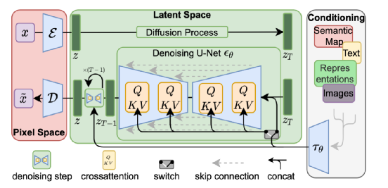
The entire model consists of three parts:
1. The leftmost Latent encoder-decoder model
Compresses the original image x into a low-dimensional latent feature z through the AutoEncoder mentioned in the previous section, while obtaining the encoderε and decoderD. To prevent the variance of z from becoming too large, making it difficult for the diffusion model to learn, a regularization term is added. One approach is the KL divergence mentioned in the VAE section (the weight of KL divergence loss should not be too large). Another approach is VQVAE, where the assumption is that z conforms to a certain discrete matrix, unlike the Gaussian continuous distribution assumed by VAE. The model architecture is as follows.
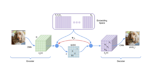
1. The expectation is that the encoder encodes z entirely within the purple embedding space depicted in the image.
2. The decoder generates images using , rather than using the encoded output from the encoder
 .
. All come from
 .
3. The control condition conditioning module on the far right
can take any input as a control condition, such as images, semantic maps, text, etc. These original conditions are processed through a pre-trained neural network
.
3. The control condition conditioning module on the far right
can take any input as a control condition, such as images, semantic maps, text, etc. These original conditions are processed through a pre-trained neural network to obtain feature representations
 , for example, the text encoder used in Stable Diffusion V1 is the CLIP text encoder, while Stable Diffusion V2 uses the OpenCLIP text encoder.
4. The middle Diffusion Model module
This uses a classifier-free diffusion model, which is fundamentally consistent with other diffusion models. In the forward diffusion process, it derives zT from z, and the model predicts noise
, for example, the text encoder used in Stable Diffusion V1 is the CLIP text encoder, while Stable Diffusion V2 uses the OpenCLIP text encoder.
4. The middle Diffusion Model module
This uses a classifier-free diffusion model, which is fundamentally consistent with other diffusion models. In the forward diffusion process, it derives zT from z, and the model predicts noise . In the reverse process, it generates latent features z, which are then decoded into images using the AutoEncoder’s decoder D.
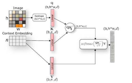
Unlike the simple addition of control conditions y in the previous DALL-E-2 and ImaGen models, this uses cross-attention for integration, allowing the varying features of y
. In the reverse process, it generates latent features z, which are then decoded into images using the AutoEncoder’s decoder D.
Unlike the simple addition of control conditions y in the previous DALL-E-2 and ImaGen models, this uses cross-attention for integration, allowing the varying features of y to serve as K and V in the attention mechanism, while the transformed features of each diffusion step
 serve as Q, making it easier to understand with the diagram below (the context embedding is
 , and the image is
 ).
).
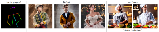
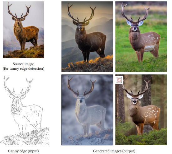
5. ControlNet
As previously mentioned, while DALL-E-2, ImaGen, LDM, and others can control image generation through conditions like text, the high degree of freedom in text semantics makes it impossible to achieve precise control, such as with lines, shapes, and image depth. Based on this limitation, ControlNet was introduced. ControlNet can introduce additional control conditions on the original LDM model through a plug-in approach, requiring only a small amount of fine-tuning data to achieve precise control over the generated images. The image below demonstrates the precise control of generated images using edge lines.
1. Basic Principle
The basic principle of ControlNet is illustrated in the image below, which introduces a residual-like module to learn new control conditions.
The left side shows the original model, which is frozen and its parameters will not be updated; the right side’s trainable copy is a copy of the left model and parameters. The core consists of two zero convolutions, which have weights and biases set to zero in a 1×1 convolution. The first zero convolution accepts new control conditions (extracted through neural networks or other techniques, such as edge lines, depth of field, etc.). At the start of training, due to the zero convolution, the features passed to y from the right training part are zero, equivalent to the output of the original LDM model.
2. Model Architecture
Based on the above principles, the improved architecture diagram of the original LDM is as follows:
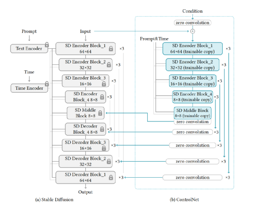
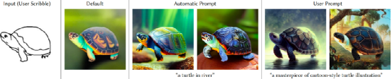
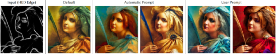
The Control module copies LDM’s down-sampling blocks and Mid Conv Blocks, with the output of each block fused through zero convolutions and corresponding blocks of LDM’s Unet during upsampling. Besides the edge lines shown earlier, other released controls include Hough lines, hand-drawn sketches, HED edges, human poses, and more.
6. References
1. https://openai.com/dall-e-2/
2. https://imagen.research.google/
3. https://arxiv.org/abs/2112.10752
4. https://arxiv.org/abs/2302.05543
5. https://openai.com/blog/clip/
6. https://arxiv.org/abs/1910.10683
7. https://www.assemblyai.com/blog/how-dall-e-2-actually-works/
8. https://web.cs.ucla.edu/~patricia.xiao/files/Win2023_Math_Reading_Group_Stable_Diffusion.pd
9. https://zhuanlan.zhihu.com/p/609075353
10. https://zhuanlan.zhihu.com/p/9143