Diffusion-TS: Interpretable Diffusion for General Time Series Generation

Introduction

Time series data is ubiquitous in various fields such as finance, healthcare, retail, and climate modeling. However, data sharing can lead to privacy breaches, limiting the development of machine learning solutions. Synthesizing realistic time series data is seen as a promising solution and has gained increasing attention with advancements in deep learning. The proposed Diffusion-TS model combines seasonal-trend decomposition techniques with the Denoising Diffusion Probabilistic Model (DDPM) and introduces a Transformer-based architecture, capable of generating high-quality time series data and performing excellently across various applications.

[Paper Title] Diffusion-TS: Interpretable Diffusion for General Time Series Generation

[Paper Link] https://openreview.net/forum?id=4h1apFjO99

[Code Link] https://github.com/Y-debug-sys/Diffusion-TS

[Affiliation/Authors] Hefei University of Technology

[Source] ICLR 2024

Abstract

This paper presents Diffusion-TS, a time series generation framework based on the Denoising Diffusion Probabilistic Model (DDPM). This framework combines seasonal-trend decomposition techniques and a Fourier-based training objective, allowing for the generation of high-quality time series data. Diffusion-TS excels in unconditional generation tasks and can also be extended to conditional generation tasks such as time series interpolation and forecasting by integrating gradient sampling methods. Experimental results show that Diffusion-TS outperforms existing generation methods across multiple time series datasets.

Innovations

1. Combination of Seasonal-Trend Decomposition and Diffusion Model: Diffusion-TS introduces seasonal-trend decomposition techniques to better capture complex patterns in time series and generate interpretable time series data.
2. Fourier-Based Training Objective: By utilizing Fourier transforms, Diffusion-TS can more accurately reconstruct time series signals in the frequency domain, thereby improving generation quality.
3. Conditional Generation Method: Diffusion-TS proposes a reconstruction-based sampling method that can flexibly apply to conditional generation tasks such as time series interpolation and forecasting without requiring parameter updates.

Methodology and Technical Details

Diffusion Model Framework

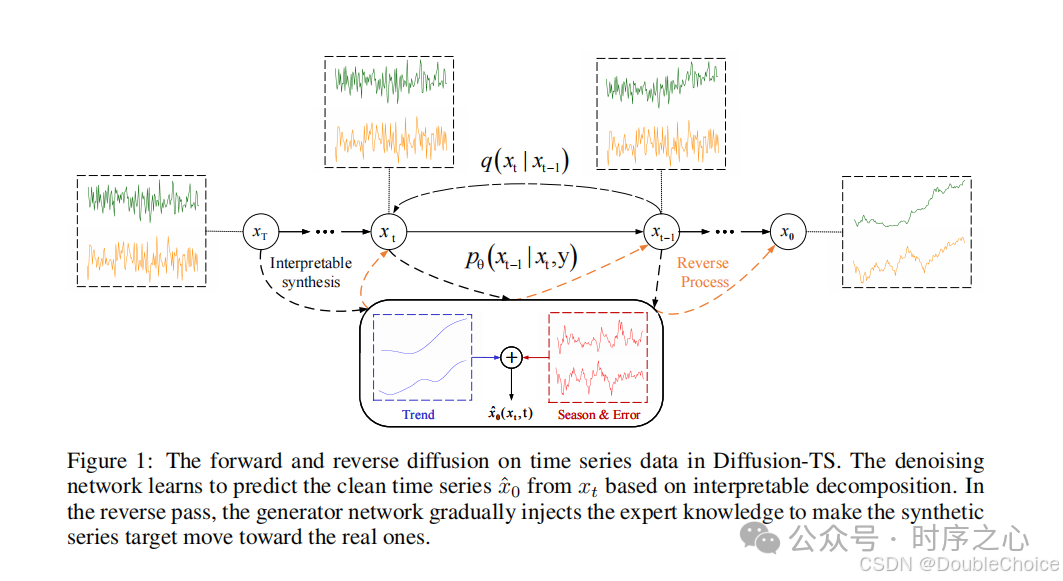
The diffusion model consists of two processes: the forward process and the reverse process. In the forward process, data samples are gradually corrupted by noise until they become standard Gaussian noise, while the reverse process progressively denoises through a neural network to generate clean samples. Specifically, the transition probability of the forward process is:

where is the amount of noise added at the diffusion step (i), and the reverse process learns the denoising process through a neural network:

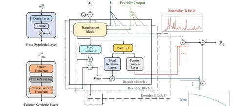
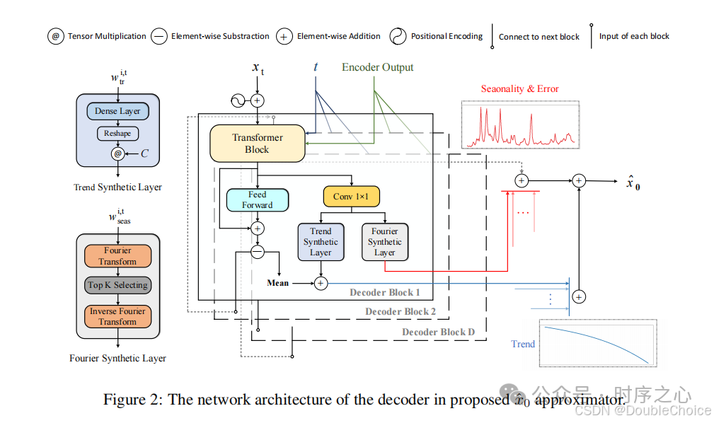
Decomposition Model Architecture

Diffusion-TS employs a Transformer-based encoder-decoder architecture. The encoder block contains a full attention mechanism and a feedforward network block, while the decoder block includes a full attention mechanism and a cross-attention mechanism to integrate encoded information. The decoder also introduces interpretable information (trend and seasonal components) to decompose the trend and seasonal components in the time series.

The trend component is modeled using a polynomial regressor:

where is the search polynomial space and is the output mean of the k-th decoder block.

The seasonal component is modeled using Fourier bases:

where and are the amplitude and phase of the k-th frequency, respectively.

Fourier-Based Training Objective

To accurately model time series signals in the frequency domain, Diffusion-TS introduces a Fourier-based training objective:

where represents the Fast Fourier Transform, and and are the weights balancing the two objectives.

Conditional Generation Method

Diffusion-TS proposes a reconstruction-based sampling method that can flexibly apply to conditional generation tasks such as time series interpolation and forecasting without needing parameter retraining. Specifically, the sampling process for conditional generation can be realized through the following formula:

where controls the strength of gradient updates and is a hyperparameter balancing conditional consistency and smoothness.

Experimental Results

Experimental results show that Diffusion-TS outperforms existing generation methods across multiple time series datasets. In unconditional generation tasks, Diffusion-TS performs excellently in metrics such as discriminative scores, predictive scores, and correlation scores. In conditional generation tasks, Diffusion-TS also excels in time series interpolation and forecasting tasks, especially under high missing rates, where its performance significantly surpasses other baseline methods.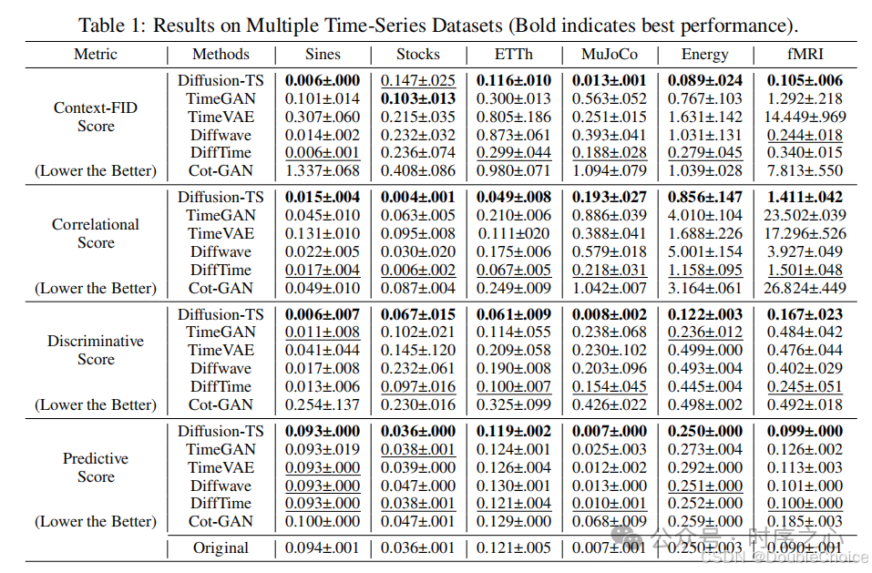MSE metrics under different missing rates in two datasets: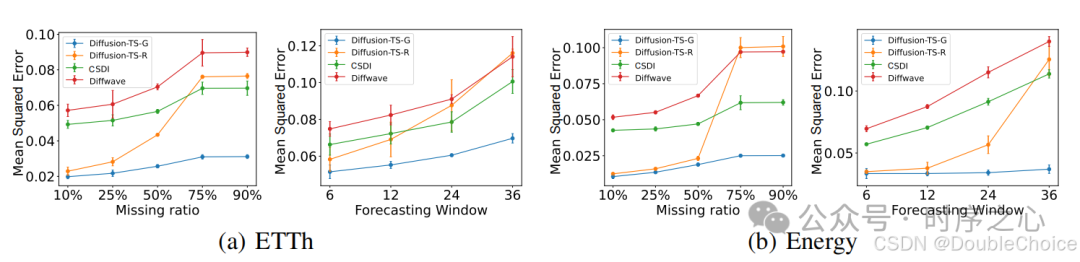Ablation experiments:

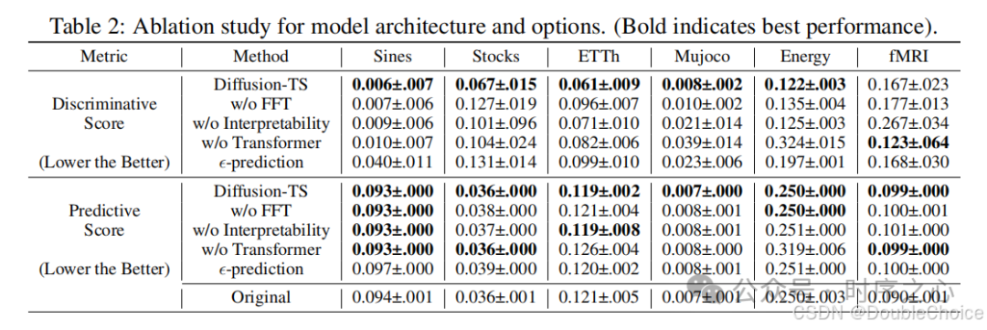
Conclusion

The Diffusion-TS model proposed in this paper, by combining seasonal-trend decomposition techniques and the Denoising Diffusion Probabilistic Model, can generate high-quality time series data. Experimental results indicate that Diffusion-TS outperforms existing generation methods across multiple time series datasets and also performs excellently in conditional generation tasks. Future work can further optimize the model’s inference efficiency to shorten generation time.

Code

Code example for the Diffusion module:

class Diffusion_TS(nn.Module):
    def __init__(
            self,
            seq_length,
            feature_size,
            n_layer_enc=3,
            n_layer_dec=6,
            d_model=None,
            timesteps=1000,
            sampling_timesteps=None,
            loss_type='l1',
            beta_schedule='cosine',
            n_heads=4,
            mlp_hidden_times=4,
            eta=0.,
            attn_pd=0.,
            resid_pd=0.,
            kernel_size=None,
            padding_size=None,
            use_ff=True,
            reg_weight=None,
            **kwargs
    ):
        super(Diffusion_TS, self).__init__()

        self.eta, self.use_ff = eta, use_ff
        self.seq_length = seq_length
        self.feature_size = feature_size
        self.ff_weight = default(reg_weight, math.sqrt(self.seq_length) / 5)

        self.model = Transformer(n_feat=feature_size, n_channel=seq_length, n_layer_enc=n_layer_enc, n_layer_dec=n_layer_dec,
                                 n_heads=n_heads, attn_pdrop=attn_pd, resid_pdrop=resid_pd, mlp_hidden_times=mlp_hidden_times,
                                 max_len=seq_length, n_embd=d_model, conv_params=[kernel_size, padding_size], **kwargs)

        if beta_schedule == 'linear':
            betas = linear_beta_schedule(timesteps)
        elif beta_schedule == 'cosine':
            betas = cosine_beta_schedule(timesteps)
        else:
            raise ValueError(f'unknown beta schedule {beta_schedule}')

        alphas = 1. - betas
        alphas_cumprod = torch.cumprod(alphas, dim=0)
        alphas_cumprod_prev = F.pad(alphas_cumprod[:-1], (1, 0), value=1.)

        timesteps, = betas.shape
        self.num_timesteps = int(timesteps)
        self.loss_type = loss_type

        # sampling related parameters

        self.sampling_timesteps = default(
            sampling_timesteps, timesteps)  # default num sampling timesteps to number of timesteps at training

        assert self.sampling_timesteps <= timesteps
        self.fast_sampling = self.sampling_timesteps < timesteps

        # helper function to register buffer from float64 to float32

        register_buffer = lambda name, val: self.register_buffer(name, val.to(torch.float32))

        register_buffer('betas', betas)
        register_buffer('alphas_cumprod', alphas_cumprod)
        register_buffer('alphas_cumprod_prev', alphas_cumprod_prev)

        # calculations for diffusion q(x_t | x_{t-1}) and others

        register_buffer('sqrt_alphas_cumprod', torch.sqrt(alphas_cumprod))
        register_buffer('sqrt_one_minus_alphas_cumprod', torch.sqrt(1. - alphas_cumprod))
        register_buffer('log_one_minus_alphas_cumprod', torch.log(1. - alphas_cumprod))
        register_buffer('sqrt_recip_alphas_cumprod', torch.sqrt(1. / alphas_cumprod))
        register_buffer('sqrt_recipm1_alphas_cumprod', torch.sqrt(1. / alphas_cumprod - 1))

        # calculations for posterior q(x_{t-1} | x_t, x_0)

        posterior_variance = betas * (1. - alphas_cumprod_prev) / (1. - alphas_cumprod)

        # above: equal to 1. / (1. / (1. - alpha_cumprod_tm1) + alpha_t / beta_t)

        register_buffer('posterior_variance', posterior_variance)

        # below: log calculation clipped because the posterior variance is 0 at the beginning of the diffusion chain

        register_buffer('posterior_log_variance_clipped', torch.log(posterior_variance.clamp(min=1e-20)))
        register_buffer('posterior_mean_coef1', betas * torch.sqrt(alphas_cumprod_prev) / (1. - alphas_cumprod))
        register_buffer('posterior_mean_coef2', (1. - alphas_cumprod_prev) * torch.sqrt(alphas) / (1. - alphas_cumprod))

        # calculate reweighting
        
        register_buffer('loss_weight', torch.sqrt(alphas) * torch.sqrt(1. - alphas_cumprod) / betas / 100)

    def predict_noise_from_start(self, x_t, t, x0):
        return (
                (extract(self.sqrt_recip_alphas_cumprod, t, x_t.shape) * x_t - x0) /
                extract(self.sqrt_recipm1_alphas_cumprod, t, x_t.shape)
        )
    
    def predict_start_from_noise(self, x_t, t, noise):
        return (
            extract(self.sqrt_recip_alphas_cumprod, t, x_t.shape) * x_t -
            extract(self.sqrt_recipm1_alphas_cumprod, t, x_t.shape) * noise
        )

    def q_posterior(self, x_start, x_t, t):
        posterior_mean = (
                extract(self.posterior_mean_coef1, t, x_t.shape) * x_start +
                extract(self.posterior_mean_coef2, t, x_t.shape) * x_t
        )
        posterior_variance = extract(self.posterior_variance, t, x_t.shape)
        posterior_log_variance_clipped = extract(self.posterior_log_variance_clipped, t, x_t.shape)
        return posterior_mean, posterior_variance, posterior_log_variance_clipped
    
    def output(self, x, t, padding_masks=None):
        trend, season = self.model(x, t, padding_masks=padding_masks)
        model_output = trend + season
        return model_output

Note: The content of this article is a sharing of insights from the paper study. Due to limitations in knowledge and ability, the understanding of the original text may be biased, and the final content is subject to the original paper. The information in this article aims for dissemination and academic exchange, and its content is the author’s responsibility, not representing the views of this account. If there are any issues regarding content, copyright, and others in the works mentioned in the text, please contact us in time, and we will respond and handle it as soon as possible.