Comprehensive Tutorial: Visualizing Transformer

Click the above “Beginner Learn Vision“, select to add “to favorites” or “pin“

Important content delivered in real-time

This article is the second part of the visual AI algorithm tutorial series, and today’s main character is Transformer.

Transformer can do many interesting and meaningful things.

For example, I previously wrote about “What is it like to play Honor of Kings with my own trained AI?”.

Another example is OpenAI‘s DALL·E, which can magically generate corresponding images directly from natural language descriptions!

Input text: An armchair in the shape of an avocado.

AI-generated image:

Both are multimodal applications, which is also the direction of major tech giants, making it a trend.

Transformer was initially mainly used in some natural language processing scenarios, such as translation, text classification, writing novels, songwriting, etc.

With the development of technology, Transformer has begun to conquer the visual field, handling tasks such as classification and detection, gradually moving towards multimodal applications.

Transformer has been very popular in the past two years, with a lot of content available. To explain it clearly, we also need to discuss some pre-trained models based on this architecture, such as the famous BERT, GPT, and the newly released DALL·E.

They are all upper-layer applications based on Transformer. Because Transformer is difficult to train, the tech giants have taken on the mission of benefiting the public by open-sourcing various useful pre-trained models.

We all learn on the shoulders of giants, using open-source pre-trained models for transfer learning in specific application scenarios.

Due to space limitations, this article will first explain the basic principles of Transformer, hoping that everyone can understand it.

I will continue to write about BERT, GPT, and other topics. The updates may be slow, but if you follow along, you will definitely gain something.

Still, as I said: If you like this AI algorithm tutorial series, please let me know, share and support, and I’ll have more motivation to write!

Transformer is a model for machine translation proposed by Google in 2017.

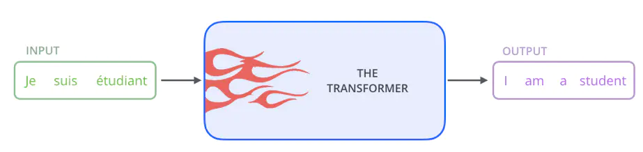
The internal structure of Transformer essentially consists of an Encoder-Decoder structure.

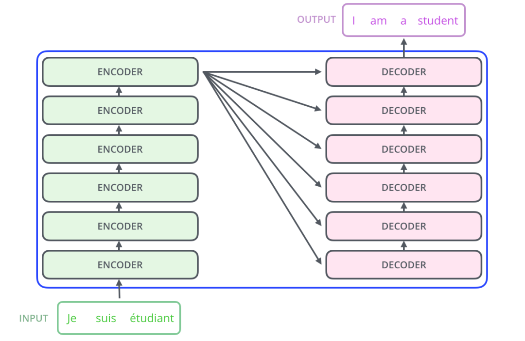
Transformer discards traditional CNN and RNN, and the entire network structure consists entirely of the Attention mechanism, using a 6 layer Encoder-Decoder structure.

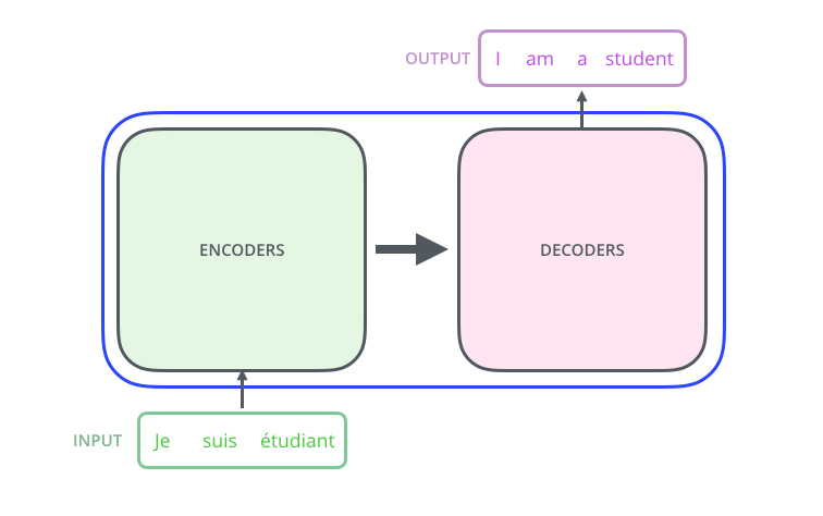
Clearly, Transformer is mainly divided into two major parts, namely encoder and decoder.

The entire Transformer consists of 6 such structures. For ease of understanding, we will only look at one Encoder-Decoder structure.

Let’s illustrate this with a simple example:

Why do we work?, why do we work?

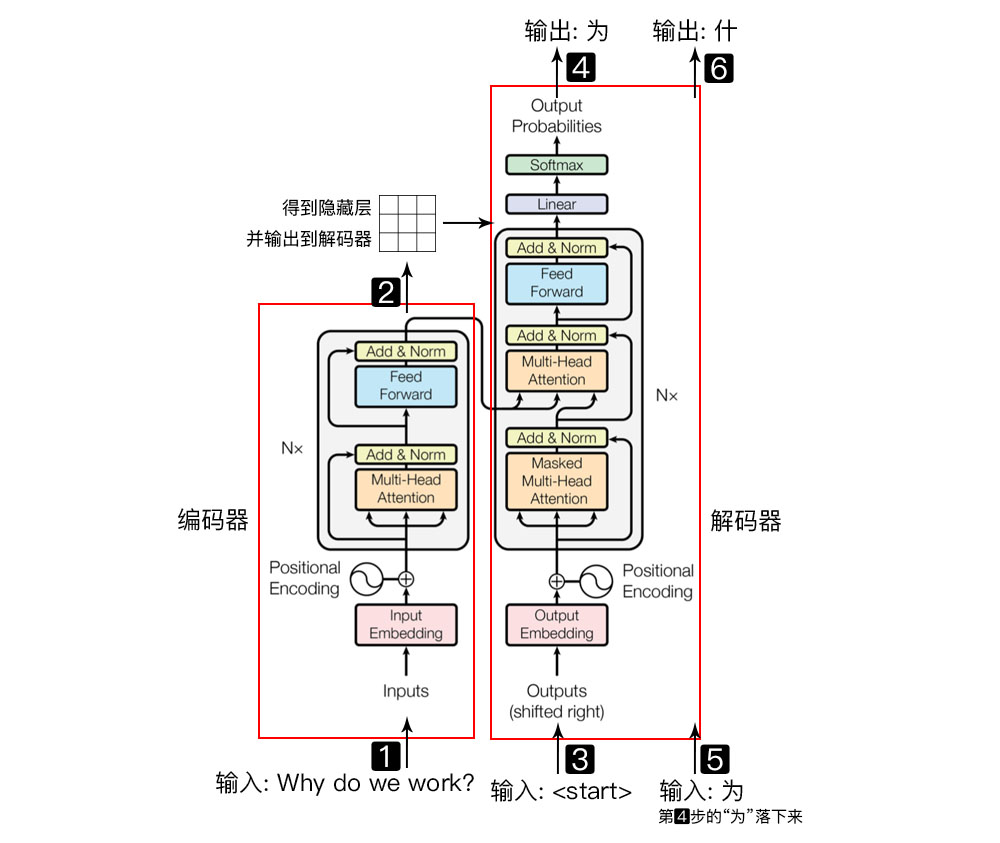
The left red box is the encoder, and the right red box is the decoder.

The encoder is responsible for mapping the natural language sequence into a hidden layer (the second step in the above figure), which contains a mathematical representation of the natural language sequence.

The decoder maps the hidden layer back into a natural language sequence, allowing us to solve various problems such as sentiment analysis, machine translation, summary generation, and semantic relationship extraction.

To briefly explain what each step in the above figure does:

• Input the natural language sequence into the encoder: Why do we work? (为什么要工作);
• The hidden layer output from the encoder is then input into the decoder;
• Input the <𝑠𝑡𝑎𝑟𝑡> (start) symbol into the decoder;
• The decoder outputs the first character “为”;
• The obtained first character “为” is then input back into the decoder;
• The decoder outputs the second character “什”;
• The obtained second character is input back until the decoder outputs <𝑒𝑛𝑑> (end symbol), completing the sequence generation.

The structures of the decoder and encoder are similar. This article will explain the encoder part, which is the process of mapping the natural language sequence to a mathematical representation of the hidden layer. Understanding the structure within the encoder makes understanding the decoder very simple.

For ease of learning, I will divide the encoder into 4 parts and explain them sequentially.

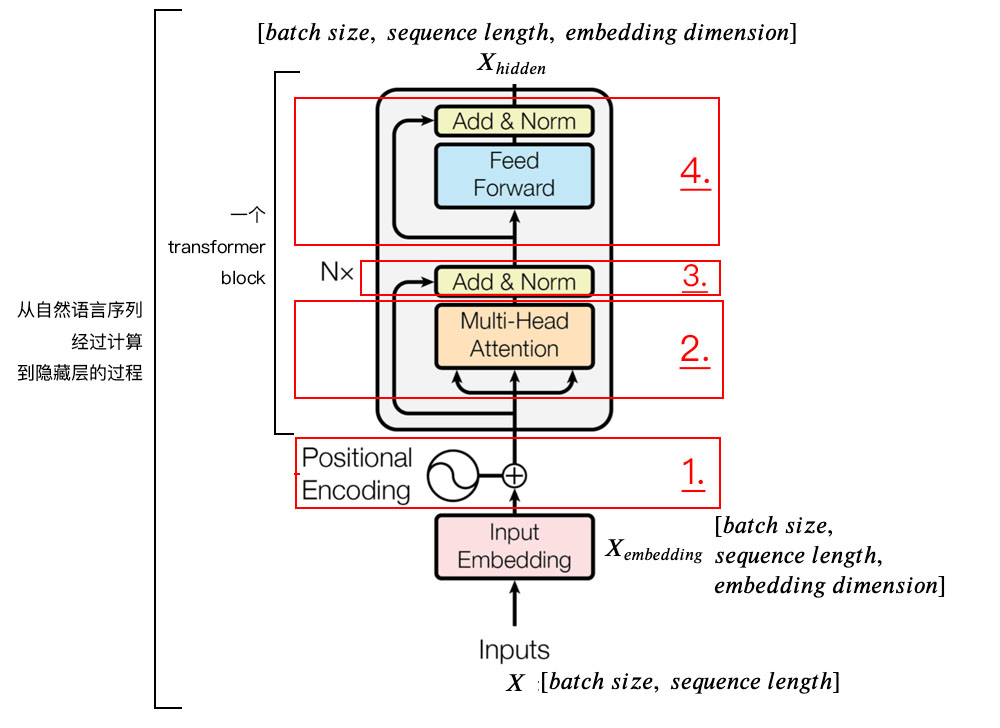
1. Positional Encoding

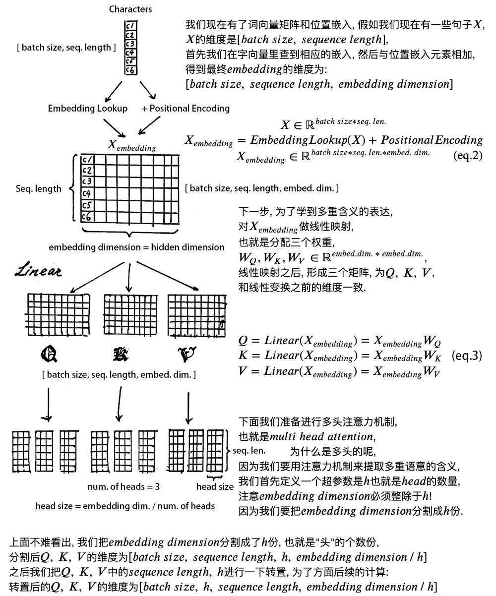
We input data X with dimensions [batch size, sequence length], for example, Why do we work?.

batch size refers to the size of the batch, and since there is only one sentence here, the batch size is 1. The sequence length is the length of the sentence, which has 7 characters, so the input data dimensions are [1, 7].

We cannot directly input this sentence into the encoder because Transformer does not understand it. We first need to perform word embedding, which is the conversion from text to vector representation.

In simpler terms, it is the conversion from words to word vectors, which is a mathematical representation that the computer can understand. The method used is Word2Vec. The specific details of Word2Vec do not need to be understood by beginners; it can be directly used.

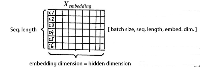
The resulting X has dimensions of [batch size, sequence length, embedding dimension], where the size of the embedding dimension is determined by the Word2Vec algorithm. Transformer uses a vector length of 512. Therefore, the dimensions of X are [1, 7, 512].

At this point, the input Why do we work? can be simplified to a matrix representation.

We know that the order of words is very important.

For example, 吃饭没, 没吃饭, 没饭吃, 饭吃没, 饭没吃, although they consist of the same three characters, the meaning changes with the order.

The positional information of words is crucial. Transformer does not have a cyclical structure like RNN, so it cannot capture the sequential nature of the input.

To retain this positional information for Transformer to learn, we need to use positional encoding.

There are many ways to incorporate positional information; the simplest method is to encode absolute coordinates 0,1,2.

Transformer uses the sin-cos rule, applying linear transformations of the sin and cos functions to provide positional information to the model:

In the above formula, pos refers to the position of the word in the sentence, with a range of [0, 𝑚𝑎𝑥 𝑠𝑒𝑞𝑢𝑒𝑛𝑐𝑒 𝑙𝑒𝑛𝑔𝑡ℎ], and i refers to the dimension of the word embedding, with a range of [0, 𝑒𝑚𝑏𝑒𝑑𝑑𝑖𝑛𝑔 𝑑𝑖𝑚𝑒𝑛𝑠𝑖𝑜𝑛]. This is the size of 𝑒𝑚𝑏𝑒𝑑𝑑𝑖𝑛𝑔 𝑑𝑖𝑚𝑒𝑛𝑠𝑖𝑜𝑛.

The above formula with sin and cos corresponds to a set of odd and even indices of the dimensions of 𝑒𝑚𝑏𝑒𝑑𝑑𝑖𝑛𝑔 𝑑𝑖𝑚𝑒𝑛𝑠𝑖𝑜𝑛, generating different periodic changes.

We can use code to see a simple effect.

# Import dependencies
import numpy as np
import matplotlib.pyplot as plt
import seaborn as sns
import math

def get_positional_encoding(max_seq_len, embed_dim):
    # Initialize a positional encoding
    # embed_dim: dimension of word embedding
    # max_seq_len: maximum sequence length
    positional_encoding = np.array([
        [pos / np.power(10000, 2 * i / embed_dim) for i in range(embed_dim)]
        if pos != 0 else np.zeros(embed_dim) for pos in range(max_seq_len)])
    positional_encoding[1:, 0::2] = np.sin(positional_encoding[1:, 0::2])  # dim 2i even
    positional_encoding[1:, 1::2] = np.cos(positional_encoding[1:, 1::2])  # dim 2i+1 odd
    # Normalize, divide each row of the positional encoding by its length
    # denominator = np.sqrt(np.sum(position_enc**2, axis=1, keepdims=True))
    # position_enc = position_enc / (denominator + 1e-8)
    return positional_encoding
    
positional_encoding = get_positional_encoding(max_seq_len=100, embed_dim=16)
plt.figure(figsize=(10,10))
sns.heatmap(positional_encoding)
plt.title("Sinusoidal Function")
plt.xlabel("hidden dimension")
plt.ylabel("sequence length")

As we can see, the positional embedding in the 𝑒𝑚𝑏𝑒𝑑𝑑𝑖𝑛𝑔 𝑑𝑖𝑚𝑒𝑛𝑠𝑖𝑜𝑛 (also hidden dimension) dimension changes periodically as the index increases, creating a texture that contains positional information.

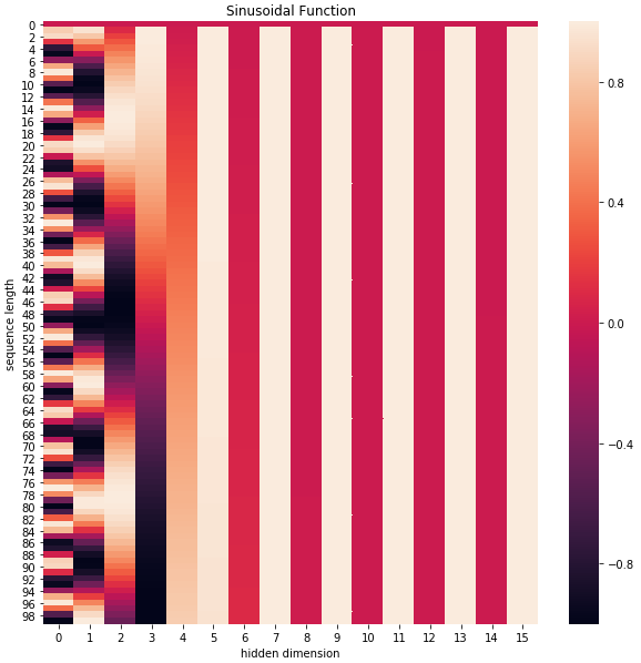
This way, unique texture positional information is generated, allowing the model to learn the dependency relationships between positions and the temporal characteristics of natural language.

Finally, X and positional encoding are added together and sent to the next layer.

2. Self-Attention Layer

Let’s look at the notes in the figure, which explain the details very well.

The significance of multi-head is that the resulting matrix is called the attention matrix, which can represent the similarity between each word and other words. Because the greater the dot product value of the vectors, the closer the two vectors are.

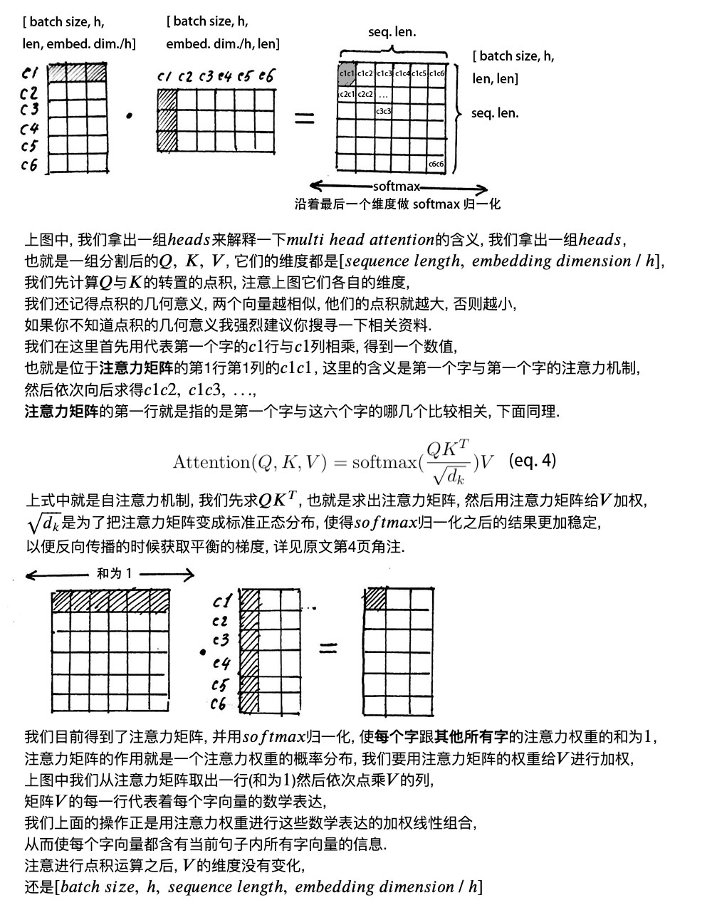
Our goal is to ensure that each word contains information from all other words in the current sentence, and we achieve this with the attention layer.

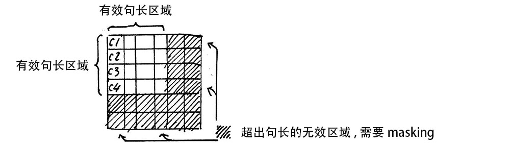
It’s important to note that during the calculation of 𝑠𝑒𝑙𝑓 𝑎𝑡𝑡𝑒𝑛𝑡𝑖𝑜𝑛, we usually use 𝑚𝑖𝑛𝑖 𝑏𝑎𝑡𝑐ℎ, meaning multiple sentences are calculated at once; the above example only used one sentence.

Each sentence has a different length, so we need to process them uniformly according to the length of the longest sentence. For shorter sentences, we perform Padding operations, usually using 0 for padding.

3. Residual Connection and Layer Normalization

Residual design and layer normalization are introduced to prevent gradient vanishing and accelerate convergence.

1) Residual Design

In the previous step, we obtained the 𝑉 weighted by the attention matrix, which is 𝐴𝑡𝑡𝑒𝑛𝑡𝑖𝑜𝑛(𝑄, 𝐾, 𝑉). We transpose it to make its dimensions consistent with 𝑋𝑒𝑚𝑏𝑒𝑑𝑑𝑖𝑛𝑔, which is [𝑏𝑎𝑡𝑐ℎ 𝑠𝑖𝑧𝑒, 𝑠𝑒𝑞𝑢𝑒𝑛𝑐𝑒 𝑙𝑒𝑛𝑔𝑡𝑕, 𝑒𝑚𝑏𝑒𝑑𝑑𝑖𝑛𝑔 𝑑𝑖𝑚𝑒𝑛𝑠𝑖𝑜𝑛], and then we add them together to perform the residual connection directly through element-wise addition, as their dimensions are consistent:

In subsequent calculations, after each module’s operation, we add the value before the operation to the value after the operation to achieve the residual connection, allowing the gradient to directly take shortcuts back to the initial layer during training:

2) Layer Normalization

The purpose is to normalize the hidden layers in the neural network to a standard normal distribution, meaning i.i.d (independent and identically distributed), to speed up training and enhance convergence.

The above formula calculates the mean based on the rows (𝑟𝑜𝑤) of the matrix:

The above formula calculates the variance based on the rows (𝑟𝑜𝑤) of the matrix:

Then, we subtract the mean of each row from each element of that row and divide by the standard deviation of that row, obtaining normalized values to prevent division;

Next, we introduce two trainable parameters to compensate for the information lost during normalization, noting that this represents element-wise multiplication rather than dot product; we generally initialize them both to one.

The code aspect is very simple; the single-head attention operation is as follows:

class ScaledDotProductAttention(nn.Module):
    ''' Scaled Dot-Product Attention '''

    def __init__(self, temperature, attn_dropout=0.1):
        super().__init__()
        self.temperature = temperature
        self.dropout = nn.Dropout(attn_dropout)

    def forward(self, q, k, v, mask=None):
        # self.temperature is d_k ** 0.5 in the paper to prevent large gradients
        # QxK/sqrt(dk)
        attn = torch.matmul(q / self.temperature, k.transpose(2, 3))

        if mask is not None:
            # Mask unwanted outputs
            attn = attn.masked_fill(mask == 0, -1e9)
        # softmax+dropout
        attn = self.dropout(F.softmax(attn, dim=-1))
        # Probability distribution x V
        output = torch.matmul(attn, v)

        return output, attn

Multi-Head Attention is implemented based on ScaledDotProductAttention:

class MultiHeadAttention(nn.Module):
    ''' Multi-Head Attention module '''

    # n_head is the number of heads, default is 8
    # d_model is the length of the encoding vector, for example, 512 as mentioned in this article
    # d_k, d_v are generally set to n_head * d_k=d_model,
    # so that after concatenation, it is exactly the same as the original input, though it can be different since there are fc layers later
    # It is equivalent to dividing the learnable matrix into n_head independent parts
    def __init__(self, n_head, d_model, d_k, d_v, dropout=0.1):
        super().__init__()
        # Suppose n_head=8, d_k=64
        self.n_head = n_head
        self.d_k = d_k
        self.d_v = d_v
        # d_model input vector, n_head * d_k output vector
        # Initialize learnable W^Q, W^K, W^V matrix parameters
        self.w_qs = nn.Linear(d_model, n_head * d_k, bias=False)
        self.w_ks = nn.Linear(d_model, n_head * d_k, bias=False)
        self.w_vs = nn.Linear(d_model, n_head * d_v, bias=False)
        # Final output dimension transformation
        self.fc = nn.Linear(n_head * d_v, d_model, bias=False)
        # Single-head self-attention
        self.attention = ScaledDotProductAttention(temperature=d_k ** 0.5)
        self.dropout = nn.Dropout(dropout)
        # Layer normalization
        self.layer_norm = nn.LayerNorm(d_model, eps=1e-6)

    def forward(self, q, k, v, mask=None):
        # Suppose qkv input is (b,100,512), where 100 is the maximum number of words per sample
        # Generally, qkv are equal, meaning self-attention
        residual = q
        # Multiply input x by learnable matrices to get (b,100,512) output
        # where 512 actually means 8x64, 8 heads, each with a 64-dimensional learnable matrix
        # The output of q is (b,100,8,64), and kv is the same
        q = self.w_qs(q).view(sz_b, len_q, n_head, d_k)
        k = self.w_ks(k).view(sz_b, len_k, n_head, d_k)
        v = self.w_vs(v).view(sz_b, len_v, n_head, d_v)

        # Reshape to (b,8,100,64) for easier calculation, meaning 8 heads compute separately
        q, k, v = q.transpose(1, 2), k.transpose(1, 2), v.transpose(1, 2)

        if mask is not None:
            mask = mask.unsqueeze(1)   # For head axis broadcasting.
        # Output q is (b,8,100,64), maintaining the same shape, internal calculation flow is:
        # q*k transpose, divided by d_k ** 0.5, output dimension is b,8,100,100, meaning the similarity between words
        # Perform softmax on the last dimension to get b,8,100,100
        # Finally multiply by V to get b,8,100,64 output
        q, attn = self.attention(q, k, v, mask=mask)

        # b,100,8,64-->b,100,512
        q = q.transpose(1, 2).contiguous().view(sz_b, len_q, -1)
        q = self.dropout(self.fc(q))
        # Residual calculation
        q += residual
        # Layer normalization, calculating mean and variance across the 512 dimensions
        q = self.layer_norm(q)

        return q, attn

4. Feed-Forward Network

This layer is straightforward, let’s look directly at the code:

class PositionwiseFeedForward(nn.Module):
    ''' A two-feed-forward-layer module '''

    def __init__(self, d_in, d_hid, dropout=0.1):
        super().__init__()
        # Two fc layers to transform the last 512 dimensions
        self.w_1 = nn.Linear(d_in, d_hid) # position-wise
        self.w_2 = nn.Linear(d_hid, d_in) # position-wise
        self.layer_norm = nn.LayerNorm(d_in, eps=1e-6)
        self.dropout = nn.Dropout(dropout)

    def forward(self, x):
        residual = x

        x = self.w_2(F.relu(self.w_1(x)))
        x = self.dropout(x)
        x += residual

        x = self.layer_norm(x)

        return x

Finally, let’s review the overall structure of the transformer encoder.

Through the above discussion, we have basically understood the main components of the transformer encoder. Next, let’s summarize the computation process of a transformer block in formula form:

1) Word vectors and positional encoding

2) Self-attention mechanism

3) Residual connection and layer normalization

4) Feed-forward network

In essence, it consists of two linear mappings followed by an activation function, for instance:

5) Repeat step 3

Thus, we have completed the discussion on the Transformer encoder, understanding how to obtain positional information in natural language and the working principle of the attention mechanism.

This article focuses on principles, and I will continue to update practical content to teach everyone how to train our own interesting and fun models.

This article is hardcore and took a long time to write. If you like it, please share and support!

I am Jack, see you next time.