In 2017, Google proposed a model called Transformer in a paper titled “Attention Is All You Need,” which is based on the attention (self-attention mechanism) structure to handle sequence-related problems.
The Transformer has achieved success in many different NLP tasks, such as text classification, machine translation, reading comprehension, etc. When solving these types of problems, the Transformer model discards inherent conventions and does not use any CNN or RNN structures, but instead utilizes the Attention mechanism to automatically capture the relative associations at different positions in the input sequence, making it adept at handling longer texts, and this model can work highly in parallel, resulting in fast training speeds.
This article will explain the Transformer module by module, introducing each module along with code + comments + explanations, and finally, there will be a toy-level sequence prediction task for practical experience.
Through this article, I hope to help everyone initially explore the principles and usage of the Transformer. Let’s dive directly into the main content:
1 Overview of Model Structure
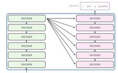
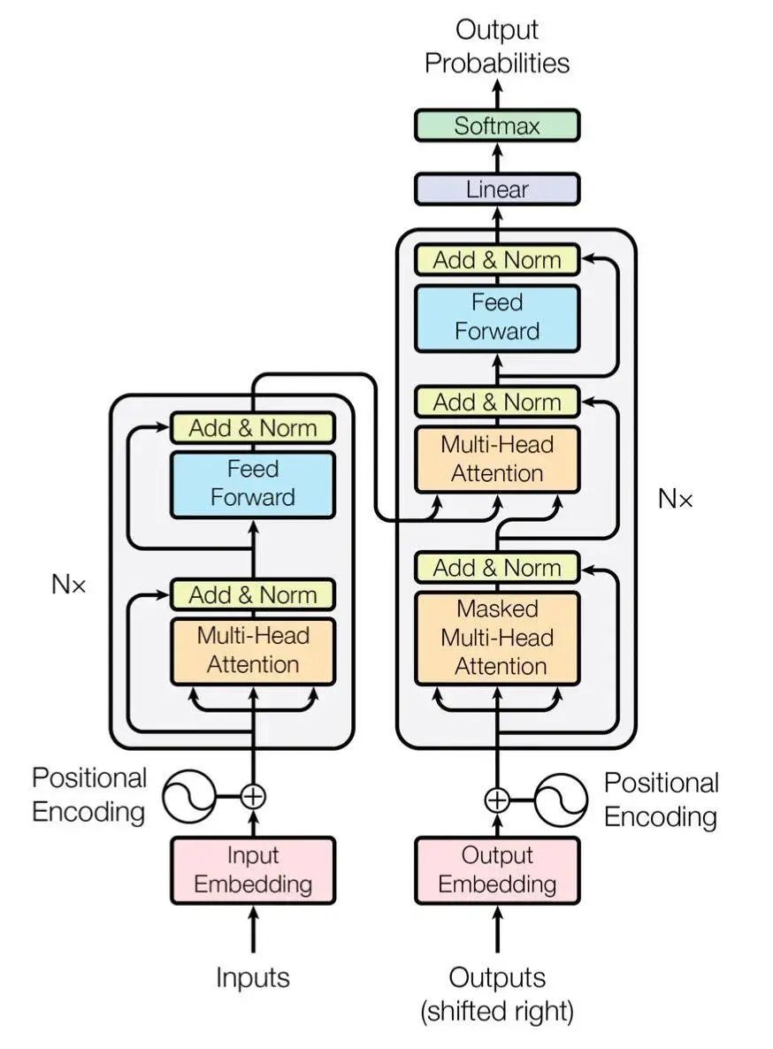
Below are two structural diagrams of the Transformer:
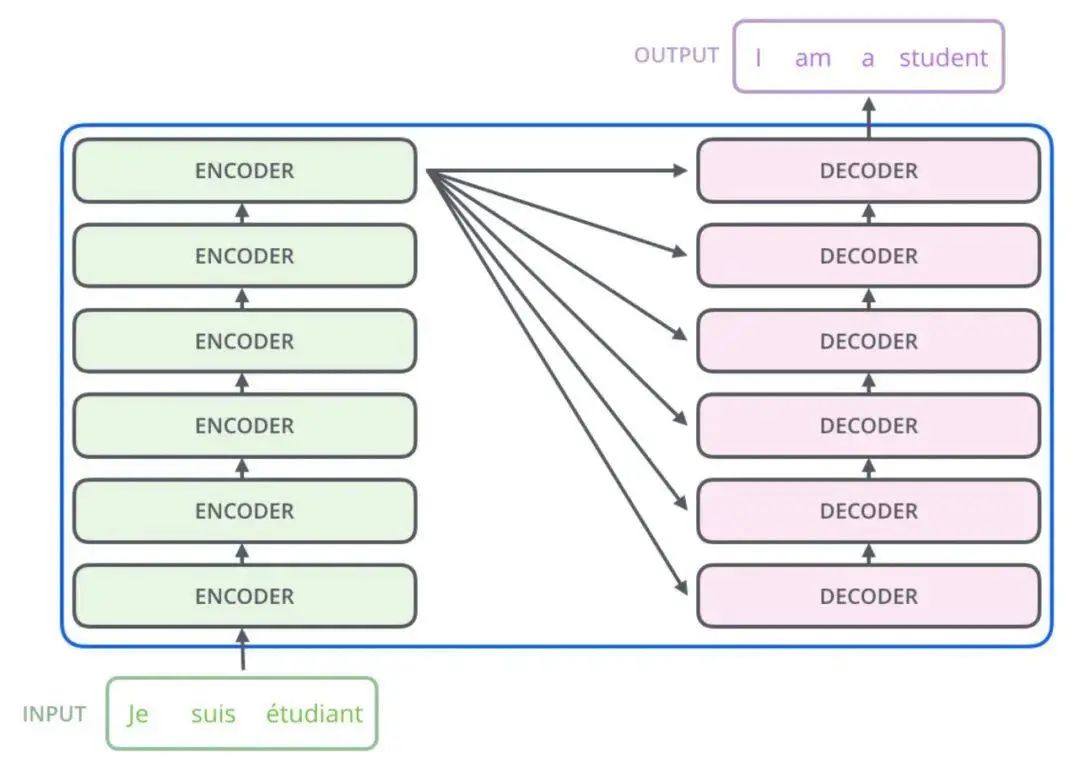
The above diagram is a simplified structure of the Transformer extracted from an English blog, and the diagram below is a more detailed structure provided in the original paper, which can be viewed together.
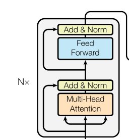
The model is roughly divided into Encoder (encoder) and Decoder (decoder), corresponding to the left and right parts of the above diagram.
The encoder consists of N identical layers stacked together (we will take N=6 in our later experiments), and each layer has two sub-layers.
The first sub-layer is a Multi-Head Attention (multi-head self-attention mechanism), and the second sub-layer is a simple Feed Forward (fully connected feedforward network). Both sub-layers add a residual connection + layer normalization operation.
The decoder also stacks N identical layers, but the structure of each layer is slightly different from that in the encoder. For each layer in the decoder, in addition to the two sub-layers Multi-Head Attention and Feed Forward from the encoder, the decoder also includes a sub-layer Masked Multi-Head Attention, as shown in the figure, where each sub-layer also uses residual connections and layer normalization.
The model input is composed of Input Embedding and Positional Encoding. The model output is simply obtained from the decoder’s output through softmax.
Combining the above diagram, we have roughly sorted out the structure of the Transformer model. We only need to have a preliminary understanding first; below we will introduce each module mentioned in detail.
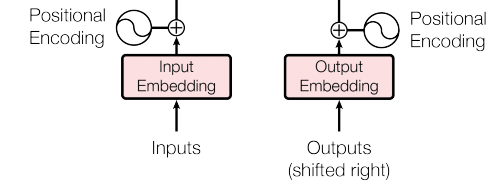
2 Model Input
First, let’s look at what the model input looks like. Clarifying the model input will make understanding the subsequent modules more intuitive.
The input part includes two modules, Embedding and Positional Encoding.
2.1 Embedding Layer
The role of the embedding layer is to convert input data of a certain format, such as text, into a vector representation that the model can process, to describe the information contained in the original data.
The output of the Embedding layer can be understood as the features at the current time step. If it is a text task, this can be Word Embedding; if it is another task, it can be any reasonable method of extracting features.
Constructing the embedding layer is quite simple, and the core is to use the nn.Embedding provided by torch, as follows:
class Embeddings(nn.Module):
    def __init__(self, d_model, vocab):
        """
        Class initialization function
        d_model: refers to the dimension of word embedding
        vocab: refers to the size of the vocabulary
        """
        super(Embeddings, self).__init__()
        # Then call the predefined layer Embedding in nn to obtain a word embedding object self.lut
        self.lut = nn.Embedding(vocab, d_model)
        # Finally, pass d_model into the class
        self.d_model =d_model
    def forward(self, x):
        """
        Forward propagation logic of the embedding layer
        Parameter x: here represents the one-hot vector obtained by mapping the input word text through the vocabulary
        Pass x to self.lut and multiply by the square root of self.d_model as the result to return
        """
        embedds = self.lut(x)
        return embedds * math.sqrt(self.d_model)
2.2 Positional Encoding:
The role of Positional Encoding is to provide the model with information about the sequential order of occurrences at the current time step. Because the Transformer does not have a cyclic structure like RNN, which has a natural order of input between different time steps, all time steps are input simultaneously and inferred in parallel. Therefore, it is reasonable to integrate positional encoding information into the features of the time steps.
Positional encoding can have many options; it can be fixed or set as learnable parameters.
Here, we use fixed positional encoding. Specifically, we use sine and cosine functions of different frequencies for positional encoding, as shown below:
Where pos represents the index of the time step, and the vector is the positional encoding of the pos-th time step, with the encoding length the same as Embedding layer, which we set to 512. The two formulas above represent the elements in the positional encoding vector, with odd and even positions using two different formulas.
Thought: Why can the above formulas serve as positional encoding?
My understanding: Under the definitions of the above formulas, the inner product of the positional encodings at time steps p and p+k is independent of p and only depends on k (you can try to prove it yourself). This means that the inner product of the positional encoding vectors at any two time steps that are k steps apart is the same, which inherently contains the relative positional relationship information between the two time steps. Additionally, the positional encoding at each time step is unique, and these two excellent properties theoretically justify the above formulas as positional encoding.
Below is the code implementation of the positional encoding module:
class PositionalEncoding(nn.Module):
    def __init__(self, d_model, dropout, max_len=5000):
        """
        Initialization function of the positional encoder class
        There are three parameters:
        d_model: word embedding dimension
        dropout: dropout trigger ratio
        max_len: maximum length of each sentence
        """
        super(PositionalEncoding, self).__init__()
        self.dropout = nn.Dropout(p=dropout)

        # Compute the positional encodings
        # Note that the calculation method in the code below is different from that in the formula, but they are equivalent; you can try to derive and prove it simply.
        # This calculation is to avoid numerical results exceeding the float range,
        pe = torch.zeros(max_len, d_model)
        position = torch.arange(0, max_len).unsqueeze(1)
        div_term = torch.exp(torch.arange(0, d_model, 2) *
                             -(math.log(10000.0) / d_model))
        pe[:, 0::2] = torch.sin(position * div_term)
        pe[:, 1::2] = torch.cos(position * div_term)
        pe = pe.unsqueeze(0)
        self.register_buffer('pe', pe)

    def forward(self, x):
        x = x + Variable(self.pe[:, :x.size(1)], requires_grad=False)
        return self.dropout(x)
Therefore, the final model input can be considered as several embeddings corresponding to the time steps, where each time step corresponds to an embedding, which can be understood as a comprehensive feature information of the current time step, containing both its own semantic information and the positional information of the current time step in the entire sentence.
2.3 Both Encoder and Decoder Contain Input Modules
Additionally, there is one point that beginners who have just come into contact with the Transformer may not understand: both the encoder and decoder parts contain inputs, and the structure of the inputs in both parts is the same; they just differ in usage during inference. The encoder infers only once, while the decoder infers in a loop similar to RNN, continuously generating prediction results.
How to understand this? Suppose we are currently performing a French-English machine translation task and want to translate Je suis étudiant into I am a student.
Then the input to the encoder will be an embedding array of length 3, and the encoder will perform a single parallel inference to obtain several feature representations for the input French sentence.
For the decoder, it is a loop inference, generating results word by word. Initially, since nothing has been predicted yet, we will pass the features extracted by the encoder along with a sentence start symbol to the decoder, which is expected to output a word I. After obtaining the first predicted word, we will input I into the decoder, which will then predict the next word am. Then we will feed I am into the decoder, and so on until we predict the sentence termination symbol to complete the prediction.
3 Encoder
This section introduces the implementation of the encoder.
3.1 Encoder
The encoder is used for feature extraction from the input, providing effective semantic information for the decoding stage.
Overall, the encoder is simply stacked from N encoder layers, so the implementation is very simple, as shown in the code below:
# Define a clones function to conveniently copy a certain structure multiple times
def clones(module, N):
    """Produce N identical layers."""
    return nn.ModuleList([copy.deepcopy(module) for _ in range(N)])


class Encoder(nn.Module):
    """
    Encoder
    The encoder is composed of a stack of N=6 identical layers.
    """
    def __init__(self, layer, N):
        super(Encoder, self).__init__()
        # When called, the encoder layer will be passed in, and we simply clone it N times, stacking them together to form the complete Encoder
        self.layers = clones(layer, N)
        self.norm = LayerNorm(layer.size)

    def forward(self, x, mask):
        """Pass the input (and mask) through each layer in turn."""
        for layer in self.layers:
            x = layer(x, mask)
        return self.norm(x)
A small detail in the above code is that the encoder’s input, in addition to x (the embedding), also includes a mask. To maintain continuity, we will ignore this for now and explain it later.
Next, let’s take a look at what each encoder layer contains and how it is implemented.
3.2 Encoder Layer
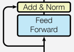
Each encoder layer consists of two sub-layer connection structures:
The first sub-layer includes a multi-head self-attention layer, a normalization layer, and a residual connection;
The second sub-layer includes a feedforward fully connected layer, a normalization layer, and a residual connection;
As shown in the figure below:
As can be seen, the structures of the two sub-layers are actually consistent; only the core layers in the middle have different implementations.
We first define a SublayerConnection class to describe this structural relationship.
class SublayerConnection(nn.Module):
    """
    Class implementing the sublayer connection structure
    """
    def __init__(self, size, dropout):
        super(SublayerConnection, self).__init__()
        self.norm = LayerNorm(size)
        self.dropout = nn.Dropout(dropout)

    def forward(self, x, sublayer):

        # Original paper's scheme
        #sublayer_out = sublayer(x)
        #x_norm = self.norm(x + self.dropout(sublayer_out))

        # Slightly adjusted version
        sublayer_out = sublayer(x)
        sublayer_out = self.dropout(sublayer_out)
        x_norm = x + self.norm(sublayer_out)
        return x_norm
Note: In the implementation above, I made a small adjustment to the residual connection scheme, which differs from the original paper. I took x out of the norm to ensure that there is always a “highway” available, which theoretically allows for faster convergence, but I cannot guarantee that this is correct, so please pay attention.
Having defined the SublayerConnection, we can now implement the EncoderLayer structure.
class EncoderLayer(nn.Module):
    """EncoderLayer is made up of two sublayers: self-attn and feed forward"""
    def __init__(self, size, self_attn, feed_forward, dropout):
        super(EncoderLayer, self).__init__()
        self.self_attn = self_attn
        self.feed_forward = feed_forward
        self.sublayer = clones(SublayerConnection(size, dropout), 2)
        self.size = size   # embedding's dimension of model, default is 512

    def forward(self, x, mask):
        # attention sub layer
        x = self.sublayer[0](x, lambda x: self.self_attn(x, x, x, mask))
        # feed forward sub layer
        z = self.sublayer[1](x, self.feed_forward)
        return z
Continuing to break it down, we need to understand the attention layer and feed_forward layer structures and how to implement them.
3.3 Attention Mechanism
When humans observe things, we cannot carefully observe everything in front of us at once; we can only focus on a particular part. Usually, after our brains quickly understand the scene in front of us, we can quickly focus our attention on the most valuable part to make effective judgments. Perhaps based on this inspiration, the idea of using attention mechanisms in algorithms arose.
Attention calculation: It requires three specified inputs Q (query), K (key), V (value), and then the attention calculation result is obtained through the following formula.
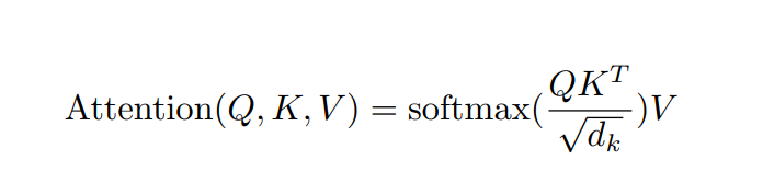
The calculation flow chart is as follows:
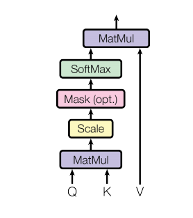
It can be simply understood that the attention calculation result at the current time step is a weighted sum of each time step’s feature vector value, where the weights are determined by the similarity between the current time step’s query and the keys of other time steps through the inner product.
Understanding the principle and thinking of the attention mechanism is worth delving into. Given the length of this article, we will focus on the code implementation here. If you are completely unfamiliar with the principles of the Transformer before reading, I recommend the following two learning resources:
Teacher Li Hongyi's Bilibili video: https://www.bilibili.com/video/BV1J441137V6?from=search&seid=3530913447603589730
DataWhale open source project: https://github.com/datawhalechina/learn-nlp-with-transformer
Below is the implementation code for the attention module:
def attention(query, key, value, mask=None, dropout=None):
    """Compute 'Scaled Dot Product Attention'"""

    # First, get the size of the last dimension of the query, corresponding to the word embedding dimension
    d_k = query.size(-1)
    # According to the attention formula, multiply the query with the transpose of the key; here, the key is transposed for the last two dimensions, and then divided by the scaling factor to obtain the attention score tensor scores
    scores = torch.matmul(query, key.transpose(-2, -1)) / math.sqrt(d_k)

    # Next, check whether to use the mask tensor
    if mask is not None:
        # Use the tensor's masked_fill method to compare each position in the mask tensor with the scores tensor; if the mask tensor is true, replace the corresponding position in the scores tensor with -1e9
        scores = scores.masked_fill(mask == 0, -1e9)

    # Perform softmax operation on the last dimension of scores, using F.softmax method, to obtain the final attention tensor
    p_attn = F.softmax(scores, dim = -1)

    # Then check whether to use dropout for random zeroing
    if dropout is not None:
        p_attn = dropout(p_attn)

    # Finally, according to the formula, multiply p_attn with the value tensor to obtain the final query attention representation, and also return the attention tensor
    return torch.matmul(p_attn, value), p_attn
3.4 Multi-Head Attention Mechanism
We just introduced the attention mechanism. The attention module used when building the EncoderLayer actually employs multi-head attention, which can be simply understood as a combination of multiple attention modules.
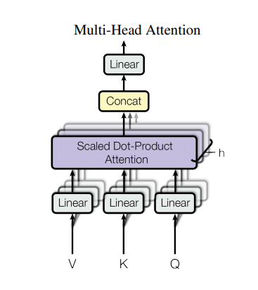
The role of the multi-head attention mechanism: This structural design allows each attention mechanism to optimize different feature parts of each word, thus balancing the biases that a single attention mechanism might produce, allowing word meanings to have more diverse expressions. Experiments have shown that this can enhance model performance.
To give a more vivid example, the word “bank” means a financial institution. If there is only one attention module, it is likely to learn to focus on words like “money” or “loan.” If we use multiple heads, different heads will focus on different semantics; for example, “bank” can also mean riverbank, so one head may focus on words like “river.” This is where the value of multi-head attention is realized.
Below is the implementation code for the multi-head attention mechanism:
class MultiHeadedAttention(nn.Module):
    def __init__(self, h, d_model, dropout=0.1):
        # In the class initialization, three parameters are passed: h represents the number of heads, d_model represents the dimension of word embeddings, and dropout represents the zeroing rate during dropout operations, default is 0.1
        super(MultiHeadedAttention, self).__init__()
        # In the function, first, use an assert statement to check whether h can be divided by d_model, because we will later allocate equal amounts of word features to each head, which is embedding_dim/head
        assert d_model % h == 0
        # Get the dimension d_k for each head
        self.d_k = d_model // h
        # Pass in the number of heads h
        self.h = h

        # Create linear layers using nn's Linear, the internal transformation matrix is embedding_dim x embedding_dim, and why four? This is because in multi-head attention, Q, K, and V each need one, and the final concatenated matrix needs one more, so there are four in total
        self.linears = clones(nn.Linear(d_model, d_model), 4)
        # self.attn is None, it represents the final attention tensor, which has no result yet, so it is None
        self.attn = None
        self.dropout = nn.Dropout(p=dropout)

    def forward(self, query, key, value, mask=None):
        # Forward logic function, which has four input parameters: the first three are Q, K, V needed for the attention mechanism, and the last one is the mask tensor that may be needed in the attention mechanism, default is None
        if mask is not None:
            # Same mask applied to all h heads.
            # Use unsqueeze to expand dimensions, representing the n-th head in multi-head
            mask = mask.unsqueeze(1)
        # Next, we get a variable nbatches, which is the first number of the query size, representing how many samples there are
        nbatches = query.size(0)

        # 1) Do all the linear projections in batch from d_model => h x d_k
        # First, use zip to group the input QKV with the three linear layers, and then use a for loop to pass the input QKV to the linear layers, perform linear transformations, and then split the input for each head using view, adding an extra dimension h for the head
        query, key, value = \
            [l(x).view(nbatches, -1, self.h, self.d_k).transpose(1, 2)
             for l, x in zip(self.linears, (query, key, value))]

        # 2) Apply attention on all the projected vectors in batch.
        # After obtaining the inputs for each head, we then pass them to the attention function, directly calling our previously implemented attention function, while also passing in the mask and dropout
        x, self.attn = attention(query, key, value, mask=mask,
                                 dropout=self.dropout)

        # 3) "Concat" using a view and apply a final linear.
        # After the multi-head attention calculation, we obtain a 4D tensor composed of the results from each head; we need to reshape it to the input shape for subsequent calculations, so here we start the inverse operation of the first step, first transposing the second and third dimensions, and then using the contiguous method. This method ensures that the transposed tensor can apply the view method; otherwise, it won't be able to use it directly. Therefore, the next step is to use view to reshape it to the same shape as the input.
        x = x.transpose(1, 2).contiguous() \
             .view(nbatches, -1, self.h * self.d_k)
        # Finally, use the last linear layer in the linear layer list to obtain the final output of the multi-head attention structure
        return self.linears[-1](x)
3.5 Feed Forward Layer
Another core sub-layer in the EncoderLayer is the Feed Forward Layer, which we will introduce here.
After performing the Attention operation, each layer in both the encoder and decoder contains a fully connected feedforward network that performs the same operation on the vector of each position, including two linear transformations and a ReLU activation output:
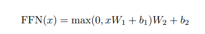
The Feed Forward Layer is simply composed of two forward fully connected layers, with the core being that the output from the Attention module integrates information from all time steps, while the Feed Forward Layer only further integrates the features of its own time step, unrelated to other time steps.
The implementation code is as follows:
class PositionwiseFeedForward(nn.Module):
    def __init__(self, d_model, d_ff, dropout=0.1):
        # The initialization function has three input parameters: d_model, d_ff, and dropout=0.1. The first is the input dimension of the linear layer, which is also the output dimension of the second linear layer, because we want the input and output dimensions to remain the same after passing through the feedforward layer. The second parameter d_ff is the input dimension of the second linear layer and the output dimension of the first linear layer, and the last parameter is the dropout zeroing rate.
        super(PositionwiseFeedForward, self).__init__()
        self.w_1 = nn.Linear(d_model, d_ff)
        self.w_2 = nn.Linear(d_ff, d_model)
        self.dropout = nn.Dropout(dropout)

    def forward(self, x):
        # The input parameter x represents the output from the previous layer. In the function, first pass through the first linear layer, then use F's relu function for activation, followed by using dropout to randomly zero, and finally pass through the second linear layer w2 to return the final result
        return self.w_2(self.dropout(F.relu(self.w_1(x))))
At this point, the main structures contained in the Encoder have all been introduced. There are two small details in the code above that have not been explained yet: layer normalization and mask, so let’s briefly explain them.
3.6 Normalization Layer
The role of the normalization layer: It is a standard network layer required by all deep network models. As the number of network layers increases, the output may begin to become too large or too small after multiple calculations, which may lead to abnormal learning processes, and the model may converge very slowly. Therefore, normalization layers are added after certain layers to normalize the numerical values, keeping them within a reasonable range.
The normalization method used in the Transformer is layer normalization, and the implementation code is quite simple, as follows:
class LayerNorm(nn.Module):
    """Construct a layernorm module (See citation for details)."""
    def __init__(self, feature_size, eps=1e-6):
        # The initialization function has two parameters: one is features, representing the embedding dimension, and the other is eps, which is a sufficiently small number that appears in the denominator of the normalization formula to prevent the denominator from being zero, default is 1e-6.
        super(LayerNorm, self).__init__()
        # Initialize two parameter tensors a2 and b2 based on the shape of features. The first is initialized to a tensor of ones, meaning all elements are ones, and the second is initialized to a tensor of zeros, meaning all elements are zeros. These two tensors are the parameters of the normalization layer. Directly normalizing the results from the previous layer will change the normal representation of the results, so parameters are needed as adjustment factors to ensure that they meet the normalization requirements without changing the representation for the target. Finally, use nn.parameter to encapsulate them, indicating that they are model parameters.
        self.a_2 = nn.Parameter(torch.ones(feature_size))
        self.b_2 = nn.Parameter(torch.zeros(feature_size))
        # Pass eps into the class
        self.eps = eps

    def forward(self, x):
        # The input parameter x represents the output from the previous layer. In the function, first compute the mean of the input variable x over the last dimension while keeping the output dimension consistent with the input dimension, then compute the standard deviation over the last dimension, and then use the normalization formula to obtain the normalized result by subtracting the mean from x and dividing by the standard deviation.
        # Finally, multiply the result by our scaling parameter, i.e., a2, where the * represents element-wise multiplication, i.e., multiplication at corresponding positions, and add the shift parameter b2 to return.
        mean = x.mean(-1, keepdim=True)
        std = x.std(-1, keepdim=True)
        return self.a_2 * (x - mean) / (std + self.eps) + self.b_2
3.7 Mask and Its Function
Mask: Mask means to cover, and code refers to the values in our tensor, which have variable dimensions and generally only contain 0 and 1; representing positions that are masked or not masked.
The role of the mask: In the transformer, the primary functions of the mask are two-fold: one is to mask out invalid padding areas, and the other is to mask out information from the “future.” The mask in the encoder primarily serves the first purpose, while the mask in the decoder serves both purposes.
Masking out invalid padding areas: When training, we need to form batches. Taking the machine translation task as an example, the input lengths of different samples in a batch are likely to be different. At this time, we need to set a maximum sentence length and pad the blank areas. The padded areas are meaningless in the calculations of both the encoder and decoder, so they need to be marked with a mask to be masked out.
Masking out information from the future: We have learned the calculation process of attention, which integrates calculations from all time steps; thus, during decoding, there is a possibility of accessing future information, which is not allowed. Therefore, this situation also requires us to use a mask for masking. If you haven’t fully understood the decoder yet, you can think about it again after we explain it.
The code for constructing the mask is as follows:
def subsequent_mask(size):
    # Generate a mask tensor that masks out subsequent positions. The parameter size represents the size of the last two dimensions of the mask tensor, which form a square matrix.

    """Mask out subsequent positions."""
    attn_shape = (1, size, size)

    # Then use np.ones to add 1 elements to this shape, forming an upper triangular matrix
    subsequent_mask = np.triu(np.ones(attn_shape), k=1).astype('uint8')

    # Finally, convert the numpy type to a torch tensor, performing a 1- operation internally. This essentially reverses the triangular matrix; each element in subsequent_mask will be reduced by 1.
    # If it is 0, the corresponding position in subsequent_mask changes from 0 to 1
    # If it is 1, the corresponding position in subsequent_mask changes from 1 to 0
    return torch.from_numpy(subsequent_mask) == 0
Above is all the content of the encoder part. With this foundation, the introduction of the decoder will be much easier.
4 Decoder
This section introduces the implementation of the decoder.
4.1 Overall Structure of the Decoder
The role of the decoder: To output the next result in the sequence based on the results of the encoder and the last predicted result.
In terms of overall structure, the decoder is also composed of N identical layers stacked together. The construction code is as follows:
# Use class Decoder to implement the decoder
class Decoder(nn.Module):
    """Generic N layer decoder with masking."""
    def __init__(self, layer, N):
        # The parameters of the initialization function are two: the first is the decoder layer layer, and the second is the number of decoder layers N
        super(Decoder, self).__init__()
        # First, use the clones method to clone N layers, then instantiate a normalization layer, because the data passes through all decoder layers and finally needs normalization processing.
        self.layers = clones(layer, N)
        self.norm = LayerNorm(layer.size)

    def forward(self, x, memory, src_mask, tgt_mask):
        # The forward function has four parameters: x represents the embedded representation of the target data, memory is the output of the encoder layer, and source_mask and target_mask represent the mask tensors for the source data and target data, respectively. Then, the input is processed through each layer in a loop, and finally normalized before returning.
        for layer in self.layers:
            x = layer(x, memory, src_mask, tgt_mask)
        return self.norm(x)
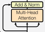
4.2 Decoder Layer
Each decoder layer consists of three sub-layer connection structures. The first sub-layer connection structure includes a multi-head self-attention sub-layer, a normalization layer, and a residual connection; the second sub-layer connection structure includes a multi-head attention sub-layer, a normalization layer, and a residual connection; the third sub-layer connection structure includes a feedforward fully connected sub-layer, a normalization layer, and a residual connection.
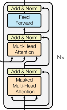
The sub-modules in the decoder layer, such as multi-head attention mechanism, normalization layer, and feedforward fully connected layer, are implemented the same as those in the encoder.
One detail to note is that the multi-head attention in the first sub-layer is identical to that in the encoder, while in the second sub-layer, the query comes from the previous sub-layer, and the keys and values come from the output of the encoder. This can be understood as the second layer utilizing the information already predicted by the decoder as the query to find relevant information from the various features extracted by the encoder and merge it into the current features to complete the prediction.
# Use the class DecoderLayer to implement the decoder layer
class DecoderLayer(nn.Module):
    """Decoder is made of self-attn, src-attn, and feed forward (defined below)"""
    def __init__(self, size, self_attn, src_attn, feed_forward, dropout):
        # The parameters of the initialization function are five: size represents the size of the word embedding, which also represents the size of the decoder; the second is self_attn, the multi-head self-attention object, meaning that this attention mechanism requires Q=K=V; the third is src_attn, the multi-head attention object, where Q != K=V; the fourth is the feedforward fully connected layer object, and the last is the dropout zeroing rate.
        super(DecoderLayer, self).__init__()
        self.size = size
        self.self_attn = self_attn
        self.src_attn = src_attn
        self.feed_forward = feed_forward
        # Clone three sub-layer connection objects according to the structure diagram
        self.sublayer = clones(SublayerConnection(size, dropout), 3)

    def forward(self, x, memory, src_mask, tgt_mask):
        # The parameters of the forward function are four: x comes from the input of the previous layer, memory is the semantic storage variable from the encoder layer, and source_mask and target_mask are the mask tensors for the source and target data, respectively. The memory is represented as m for convenience.
        """Follow Figure 1 (right) for connections."""
        m = memory
        # Pass x to the first sub-layer structure, where the input of the first sub-layer structure is x and the self-attn function, because it is a self-attention mechanism, so Q, K, V are all x, and the last parameter is the target data mask tensor, which needs to mask the target data because the model may not have generated any target data yet.
        # For example, when the decoder is about to generate the first character or word, we actually pass in the first character to calculate the loss, but we do not want the model to use this information when generating the first character; therefore, we will mask it. Similarly, when generating the second character or word, the model can only use the information from the first character or word, and the second character and subsequent information are not allowed to be used.
        x = self.sublayer[0](x, lambda x: self.self_attn(x, x, x, tgt_mask))
        # Next, enter the second sub-layer. In this sub-layer, the attention mechanism is conventional, where q is the input x; k and v are the output from the encoder layer memory. The source_mask is also passed in, but the purpose of masking the source data is not to suppress information leakage but to mask out padding that is meaningless to the result.
        x = self.sublayer[1](x, lambda x: self.src_attn(x, m, m, src_mask))

        # The last sub-layer is the feedforward fully connected sub-layer. After processing, it can return the result, which is our decoder structure.
        return self.sublayer[2](x, self.feed_forward)
5 Model Output
The output part is very simple; each time step passes through a linear layer + softmax layer.
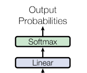
The role of the linear layer: It transforms the output from the previous step to obtain an output of the specified dimension, which serves to convert dimensions. The converted dimension corresponds to the number of output categories; if it is a translation task, it corresponds to the size of the character dictionary.
The code is as follows:
# Implement the linear layer and softmax calculation layer together since their common goal is to generate the final structure
# Thus, the class is named Generator, the generator class
class Generator(nn.Module):
    """Define standard linear + softmax generation step."""
    def __init__(self, d_model, vocab):
        # The input parameters of the initialization function are two: d_model represents the word embedding dimension, and vocab.size represents the vocabulary size
        super(Generator, self).__init__()
        # First, instantiate a predefined linear layer in nn to obtain an object self.proj for later use
        # This linear layer has two parameters: d_model and vocab_size, which are the two parameters passed into the initialization function
        self.proj = nn.Linear(d_model, vocab)

    def forward(self, x):
        # In the forward logic function, the input is the output tensor x from the previous layer. In the function, first use the previous result self.proj to perform linear transformation on x, and then use F's log_softmax for softmax processing.
        return F.log_softmax(self.proj(x), dim=-1)
6 Model Construction
Below is the overall architecture diagram of the Transformer. After reviewing this diagram, doesn’t it seem that there is a basic understanding of the role of each module?

Now we can build the entire network structure.
# Model Architecture
# Use the EncoderDecoder class to implement the encoder-decoder structure
class EncoderDecoder(nn.Module):
    """
    A standard Encoder-Decoder architecture.
    Base for this and many other models.
    """
    def __init__(self, encoder, decoder, src_embed, tgt_embed, generator):
        # The initialization function has five parameters: the encoder object, the decoder object, the source data embedding function, the target data embedding function, and the output category generator object.
        super(EncoderDecoder, self).__init__()
        self.encoder = encoder
        self.decoder = decoder
        self.src_embed = src_embed    # input embedding module(input embedding + positional encode)
        self.tgt_embed = tgt_embed    # output embedding module
        self.generator = generator    # output generation module

    def forward(self, src, tgt, src_mask, tgt_mask):
        """Take in and process masked src and target sequences."""
        # In the forward function, there are four parameters: source represents the source data, target represents the target data, and source_mask and target_mask represent the corresponding mask tensors. In the function, the source and source_mask are passed to the encoding function to obtain the results, which are then passed to the decoding function along with source_mask, target, and target_mask.
        memory = self.encode(src, src_mask)
        res = self.decode(memory, src_mask, tgt, tgt_mask)
        return res

    def encode(self, src, src_mask):
        # Encoding function, taking source and source_mask as parameters, using src_embed to process the source, then passing it along with source_mask to self.encoder
        src_embedds = self.src_embed(src)
        return self.encoder(src_embedds, src_mask)

    def decode(self, memory, src_mask, tgt, tgt_mask):
        # Decoding function, taking memory (the output of the encoder), source_mask, target, and target_mask as parameters, using tgt_embed to process the target, then passing it to self.decoder along with source_mask and target_mask
        target_embedds = self.tgt_embed(tgt)
        return self.decoder(target_embedds, memory, src_mask, tgt_mask)


# Full Model

def make_model(src_vocab, tgt_vocab, N=6, d_model=512, d_ff=2048, h=8, dropout=0.1):
    """
    Build the model
    params:
        src_vocab:
        tgt_vocab:
        N: Number of stacked base modules in the encoder and decoder
        d_model: Size of the embedding in the model, default is 512
        d_ff: Size of the embedding in the FeedForward Layer, default is 2048
        h: Number of heads in MultiHeadAttention, must be divisible by d_model
        dropout:
    """
    c = copy.deepcopy
    attn = MultiHeadedAttention(h, d_model)
    ff = PositionwiseFeedForward(d_model, d_ff, dropout)
    position = PositionalEncoding(d_model, dropout)
    model = EncoderDecoder(
        Encoder(EncoderLayer(d_model, c(attn), c(ff), dropout), N),
        Decoder(DecoderLayer(d_model, c(attn), c(attn), c(ff), dropout), N),
        nn.Sequential(Embeddings(d_model, src_vocab), c(position)),
        nn.Sequential(Embeddings(d_model, tgt_vocab), c(position)),
        Generator(d_model, tgt_vocab))

    # This was important from their code.
    # Initialize parameters with Glorot / fan_avg.
    for p in model.parameters():
        if p.dim() > 1:
            nn.init.xavier_uniform_(p)
    return model
7 Practical Case
Below we will use a small toy-level task to practically experience the training of the Transformer, deepening our understanding and verifying whether the code we described above works.
Task description: Learn to output the same sequence as the input sequence after deleting the first character, for example, if the input is [1,2,3,4,5], we try to let the model learn to output [2,3,4,5].
Clearly, this should not be difficult for the model, and it should learn quickly after several iterations.
The basic steps for implementing the code are:
Step 1: Construct and generate an artificial dataset
Step 2: Construct the Transformer model and related preparations
Step 3: Run the model for training and evaluation
Step 4: Use the model for greedy decoding
Due to space constraints, we will not introduce the code for data construction here. If you are interested, feel free to check the project source code and run it yourself: https://github.com/datawhalechina/dive-into-cv-pytorch/tree/master/code/chapter06_transformer/6.1_hello_transformer
The general training process is as follows:
# Train the simple copy task.
device = "cuda"
nrof_epochs = 20
batch_size = 32
V = 11    # Size of the vocabulary
sequence_len = 15  # Length of the generated sequence data
nrof_batch_train_epoch = 30    # Number of batches per epoch during training
nrof_batch_valid_epoch = 10    # Number of batches per epoch during validation
criterion = LabelSmoothing(size=V, padding_idx=0, smoothing=0.0)
model = make_model(V, V, N=2)
optimizer = torch.optim.Adam(model.parameters(), lr=0, betas=(0.9, 0.98), eps=1e-9)
model_opt = NoamOpt(model.src_embed[0].d_model, 1, 400, optimizer)
if device == "cuda":
    model.cuda()

for epoch in range(nrof_epochs):
    print(f"\nepoch {epoch}")
    print("train...")
    model.train()
    data_iter = data_gen(V, sequence_len, batch_size, nrof_batch_train_epoch, device)
    loss_compute = SimpleLossCompute(model.generator, criterion, model_opt)
    train_mean_loss = run_epoch(data_iter, model, loss_compute, device)
    print("valid...")
    model.eval()
    valid_data_iter = data_gen(V, sequence_len, batch_size, nrof_batch_valid_epoch, device)
    valid_loss_compute = SimpleLossCompute(model.generator, criterion, None)
    valid_mean_loss = run_epoch(valid_data_iter, model, valid_loss_compute, device)
    print(f"valid loss: {valid_mean_loss}")
After training the model, we use the greedy decoding strategy for prediction.
The method to obtain predicted results is not unique; greedy decoding is the most commonly used. We have already introduced it in the section on model input in 6.1.2, which essentially starts from a sentence start symbol, and each time infers the decoder to obtain an output, then adds the obtained output to the input of the decoder, and continues to infer until the sentence termination symbol is predicted, at which point all predictions are concatenated to get the complete prediction result.
The code for greedy decoding is as follows:
# greedy decode
def greedy_decode(model, src, src_mask, max_len, start_symbol):
    memory = model.encode(src, src_mask)
    # ys represents the currently generated sequence, initially containing only a sequence with the start symbol, which is continuously appended with predicted results at the end
    ys = torch.ones(1, 1).fill_(start_symbol).type_as(src.data)
    for i in range(max_len-1):
        out = model.decode(memory, src_mask,
                           Variable(ys),
                           Variable(subsequent_mask(ys.size(1)).type_as(src.data)))
        prob = model.generator(out[:, -1])
        _, next_word = torch.max(prob, dim = 1)
        next_word = next_word.data[0]
        ys = torch.cat([ys, torch.ones(1, 1).type_as(src.data).fill_(next_word)], dim=1)
    return ys

print("greedy decode")
model.eval()
src = Variable(torch.LongTensor([[1,2,3,4,5,6,7,8,9,10]])).cuda()
src_mask = Variable(torch.ones(1, 1, 10)).cuda()
pred_result = greedy_decode(model, src, src_mask, max_len=10, start_symbol=1)
print(pred_result[:, 1:])
Running our training script, the training process and predicted results are printed as follows:
...

epoch 18
train...
Epoch Step: 1 Loss: 0.078836 Tokens per Sec: 13734.076172
valid...
Epoch Step: 1 Loss: 0.029015 Tokens per Sec: 23311.662109
valid loss: 0.03555255010724068

epoch 19
train...
Epoch Step: 1 Loss: 0.042386 Tokens per Sec: 13782.227539
valid...
Epoch Step: 1 Loss: 0.022001 Tokens per Sec: 23307.326172
valid loss: 0.014436692930758

greedy decode
tensor([[ 2,  3,  4,  5,  6,  7,  8,  9, 10]], device='cuda:0')
As we can see, since the task is very simple, after 20 epochs of simple training, the loss has converged to a very low level.
The test case [1,2,3,4,5,6,7,8,9,10] predicts the result [2,3,4,5,6,7,8,9,10], which meets expectations, indicating that our Transformer model is correctly constructed and successful~
Summary
This time we introduced the basic principles of the Transformer, and gradually dismantled each module from the outside in, explaining the principles and code. Finally, we practiced the training and inference process of the Transformer through a toy-level demo. I hope that through these contents, beginners can have a clearer understanding of the Transformer.
This article references: http://nlp.seas.harvard.edu/2018/04/03/attention.html