
Source | Zhihu
Address | https://zhuanlan.zhihu.com/p/79872507
Author | Machine Heart
Editor | Machine Learning Algorithms and Natural Language Processing Public Account
This article is for academic sharing only, if there is any infringement, please contact us to delete it.
In the first part of this series, we reviewed the basic working principles of the Transformer and gained a preliminary understanding of the internal structure of GPT-2. In this article, we will detail the self-attention mechanism used by GPT-2 and share exciting applications of the transformer model that only contains a decoder.
Excerpted from github.io, author: Jay Alammar, compiled by Machine Heart, contributors: Chen Yunying, Geek AI.
Part Two: Illustrated Self-Attention Mechanism
In the previous article, we used this image to showcase the application of the self-attention mechanism in processing the word “it”:
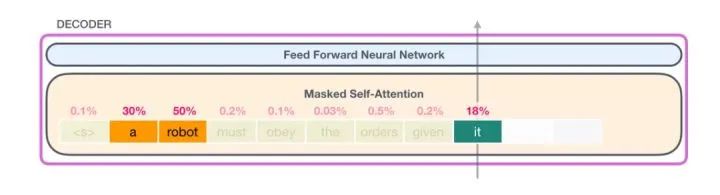
In this section, we will explain how this process is implemented in detail. Please note that we will attempt to clarify how a single word is processed. This is also the reason why we will showcase many individual vectors. This is actually achieved by multiplying giant matrices. However, I want to visualize what happens at the word level.
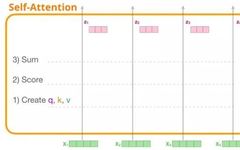
Self-Attention Mechanism (Without Masking)
First, we will introduce the original self-attention mechanism, which is computed in the encoder module. Let’s look at a simple transformer module that can only process 4 words (tokens) at a time.
The self-attention mechanism is implemented through the following three main steps:
1. Create query, key, and value vectors for each path.
2. For each input word, calculate the attention score by multiplying its query vector with all other key vectors.
3. Multiply the value vectors by their corresponding attention scores and sum them up.

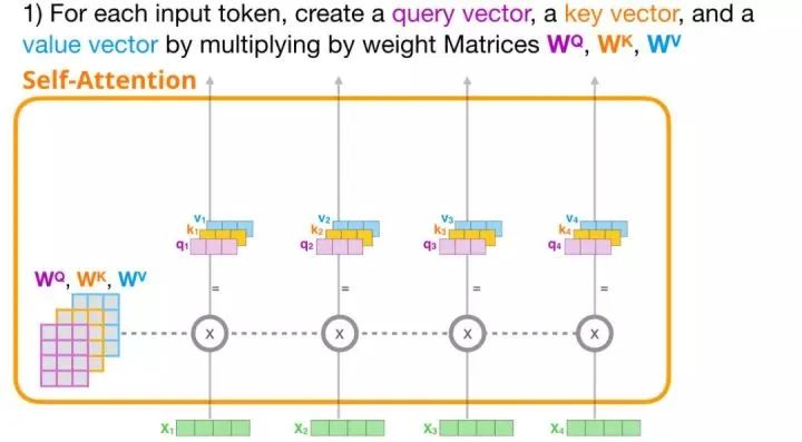
1. Create Query, Key, and Value Vectors
We focus on the first path. We compare its query value with all other key vectors, giving each key vector a corresponding attention score. The first step of the self-attention mechanism is to compute three vectors for each word (token) path (we will temporarily ignore the attention heads): query vector, key vector, and value vector.
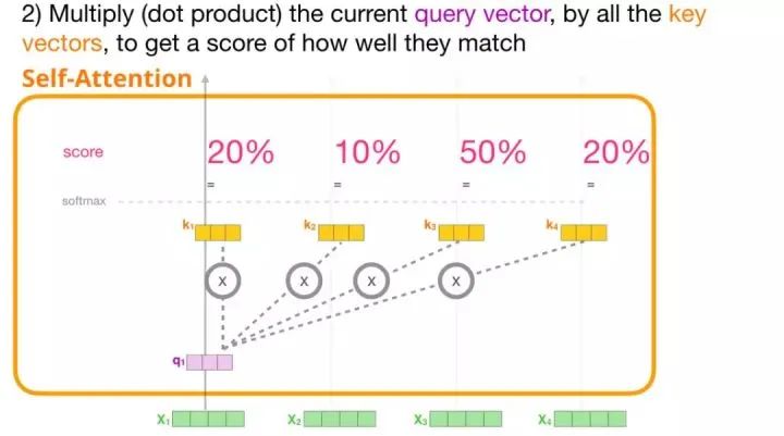
2. Attention Scores
After calculating the three vectors mentioned above, we use only the query and key vectors in the second step. We focus on the first word, multiplying its query vector with all other key vectors to obtain the attention scores for each word among the four words.
3. Summation
Now, we can multiply the attention scores with the value vectors. After summing them up, the values with higher attention scores will have a greater weight in the resulting vector.
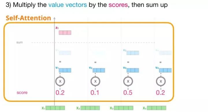
The lower the attention score, the more transparent the value vector shown in the figure. This is to illustrate how multiplying by a small number weakens the influence of the vector value.
If we perform the same operation on each path, we will ultimately obtain a vector representing each word, which includes the appropriate context for that word, and then pass this information to the next sub-layer (feed-forward neural network) in the transformer module:
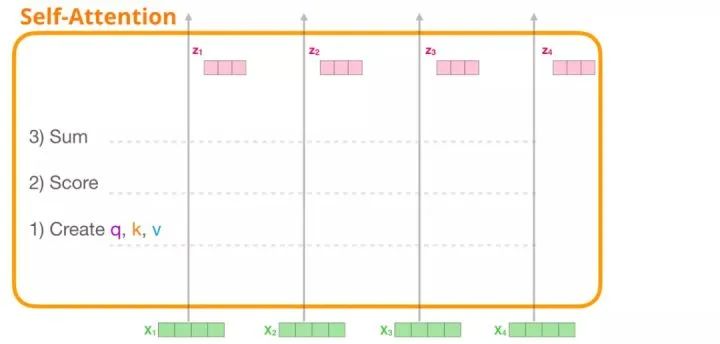
Illustration of Masked Self-Attention Mechanism
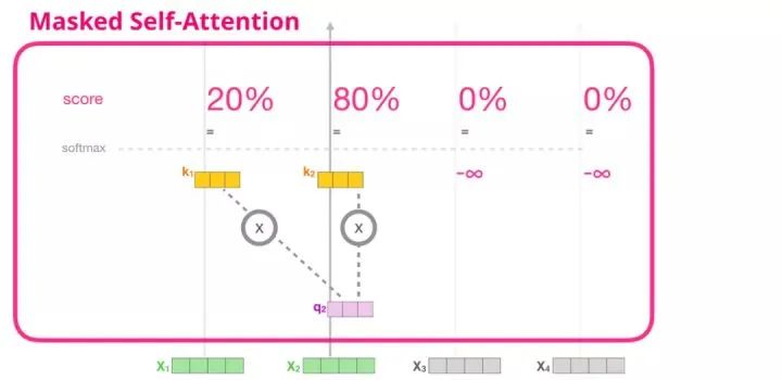
Now that we have introduced the steps of the self-attention mechanism in the transformer module, we will introduce the masked self-attention mechanism. In the masked self-attention mechanism, all parts except the second step are the same as the self-attention mechanism. Suppose the model input contains only two words, and we are observing the second word. In this case, the last two words are masked. Therefore, the model will interfere with the step of calculating the attention scores. Essentially, it always assigns a score of 0 to the attention scores of subsequent words in the sequence, so the model does not get the highest attention score for the subsequent words:
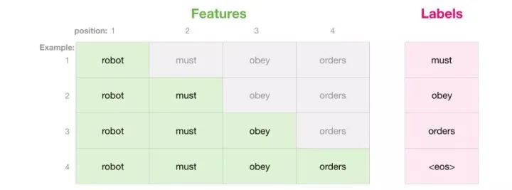
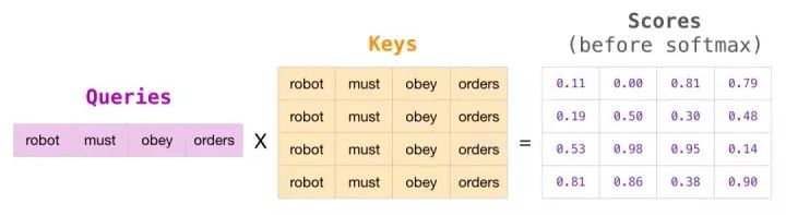
We typically use an attention mask matrix to implement this masking operation. Imagine a sequence of four words (for example, “robot must obey orders”) in a language modeling scenario, where this sequence is processed in four steps—one word at a time (assuming each word is a token). Since these models are batch executed, we assume that the batch size of this small model is 4, and it takes the entire sequence (including 4 steps) as one batch.
In matrix form, we calculate the attention scores by multiplying the query matrix by the key matrix. The visualization of this process is shown below, using the query (or key) vector associated with the word in that cell, rather than the word itself:
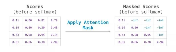
After multiplying, we add the attention mask triangular matrix. It sets the cells we want to mask to negative infinity or a very large negative number (for example, -1 billion in GPT-2):
Then, we perform the softmax operation on each row, thereby obtaining the attention scores that we actually use in the self-attention mechanism:
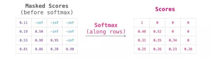
The meaning of this score table is as follows:
-
When the model processes the first example in the dataset (the first row), it only contains one word (“robot”), so 100% of the attention is on that word.
-
When the model processes the second example in the dataset (the second row), it contains (“robot must”), when it processes the word “must”, 48% of the attention is on “robot”, and the other 52% of the attention is on “must”.
-
And so on.
Masked Self-Attention Mechanism of GPT-2
Next, we will analyze the masked self-attention mechanism of GPT-2 in more detail.
1. Model Evaluation: Processing One Word at a Time
We can execute GPT-2 by means of the masked self-attention mechanism. However, during model evaluation, when our model adds one new word after each iteration, recalculating the self-attention of the words (tokens) along the previously processed paths is extremely inefficient.
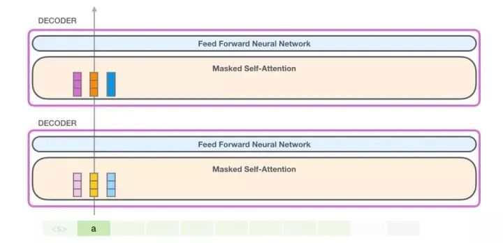
In this case, we process the first word (temporarily ignoring <s>)
GPT-2 retains the key and value vectors of the word “a”. Each self-attention layer includes the corresponding key and value vectors for that word.
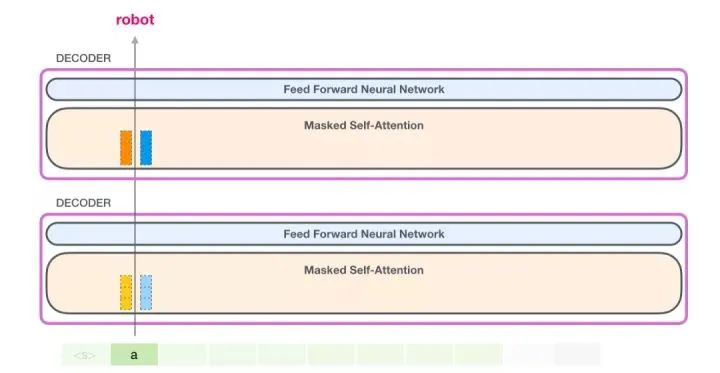
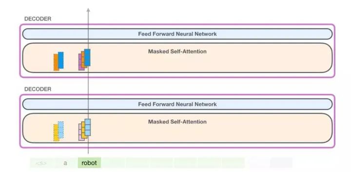
In the next iteration, when the model processes the word “robot”, it no longer needs to generate query, key, and value vectors for the word “a”. It only needs to reuse the vectors saved in the first iteration:
Now, in the next iteration, when the model processes the word “robot”, it no longer needs to generate query, key, and value vectors for the token “a”. It only needs to reuse the vectors saved in the first iteration:
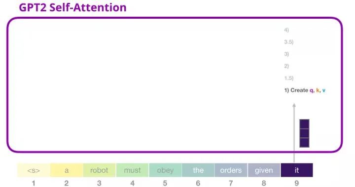
2. GPT-2 Self-Attention Mechanism: 1-Create Query, Key, and Value
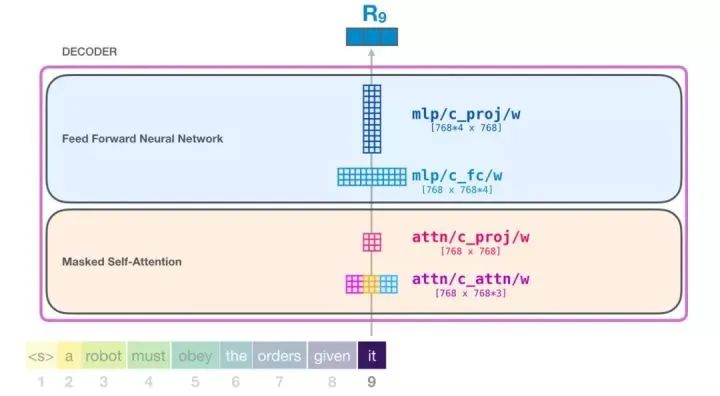
Assuming the model is processing the word “it”. For the module at the bottom of the image, its input is the embedding vector of “it” + the positional encoding of the ninth position in the sequence:
Each module in the transformer has its own weights (which will be analyzed in detail later). We first see the weight matrices used to create the query, key, and value.
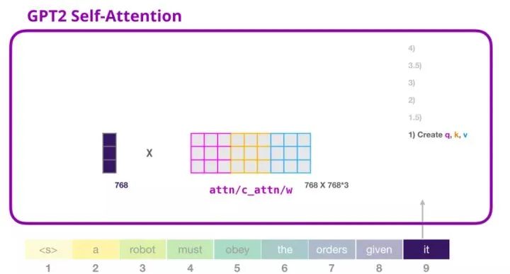
The self-attention mechanism multiplies its input by the weight matrix (and adds a bias vector, which is not illustrated here).
The resulting vector from this multiplication is essentially the concatenation of the query, key, and value vectors for the word “it”.
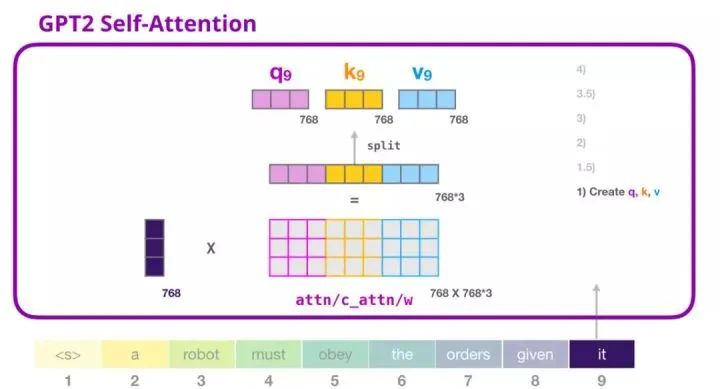
Multiplying the input vector with the attention weight vector (and then adding the bias vector) yields the key, value, and query vectors for this word.
3. GPT-2 Self-Attention Mechanism: 1.5-Split into Attention Heads
In the previous example, we introduced the self-attention mechanism while ignoring the “multi-head” part. Now, understanding this part will be useful. The self-attention mechanism operates multiple times on different parts of the query (Q), key (K), and value (V) vectors. “Splitting” attention heads refers to simply reshaping the long vector into matrix form. In the small GPT-2, there are 12 attention heads, so this is the first dimension of the reshaped matrix:
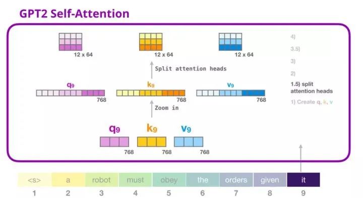
In the previous example, we introduced the case of a single attention head. Multiple attention heads can be imagined like this (the following image shows a visualization of 3 out of 12 attention heads):

4. GPT-2 Self-Attention Mechanism: 2-Calculate Attention Scores
Next, we introduce the process of calculating attention scores—at this point, we focus on a single attention head (other attention heads perform similar operations).
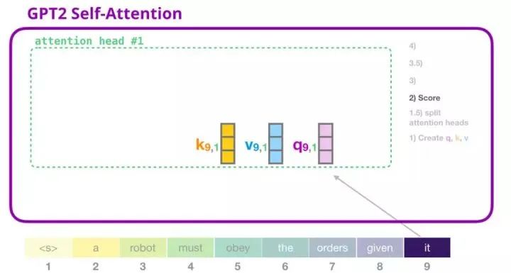
The currently focused word (token) can multiply with the key vectors of other key words to obtain attention scores (calculated in the first attention head from previous iterations):
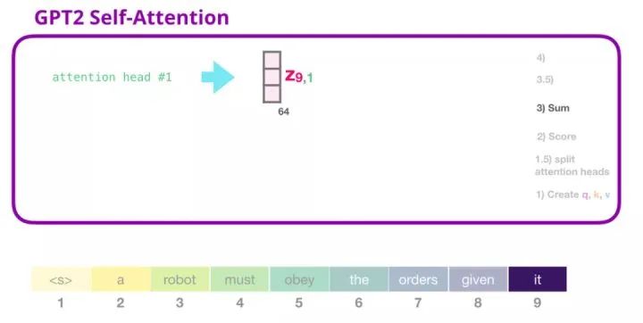
5. GPT-2 Self-Attention Mechanism: 3-Summation
As mentioned earlier, we can now multiply each value vector by its attention score and then sum them up to obtain the self-attention result of the first attention head:
6. GPT-2 Self-Attention Mechanism: 3.5-Merge Multiple Attention Heads
We handle multiple attention heads by first concatenating them into a single vector:
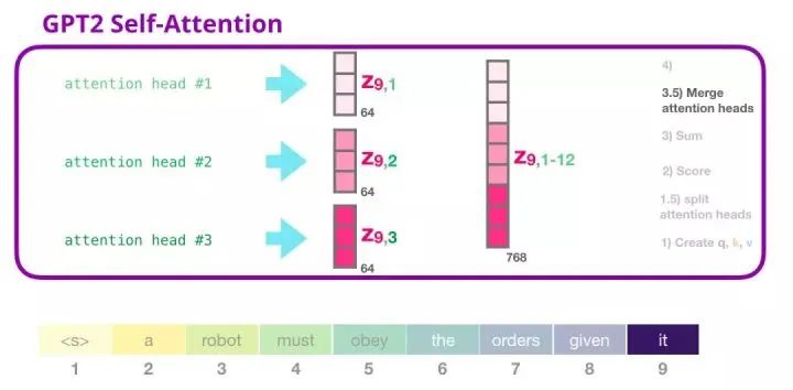
However, this vector cannot be passed to the next sub-layer yet. We first need to transform this mixed vector of hidden states into a homogeneous representation.
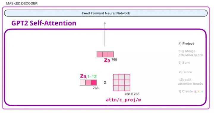
7. GPT-2 Self-Attention Mechanism: 4-Projection
We will let the model learn how best to map the connected self-attention results to a vector that can be processed by a feed-forward neural network. The following is our second large weight matrix, which projects the results of the attention heads into the output vector of the self-attention sub-layer:
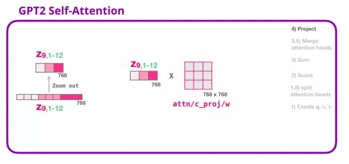
Through this operation, we can generate a vector that can be passed to the next layer:
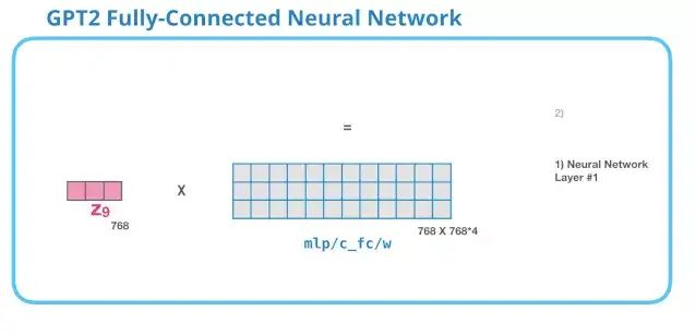
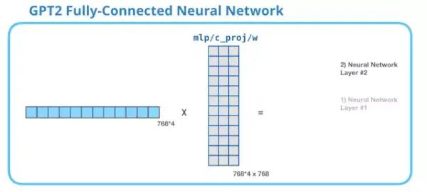
8. GPT-2 Fully Connected Neural Network: First Layer
In the fully connected neural network, after the self-attention mechanism has included the appropriate context in its representation, the module processes its input word. It consists of two layers: the size of the first layer is 4 times the model size (because the small GPT-2 has 768 units, and this network will have 768*4=3072 units). Why is it 4 times? This is simply the operational size of the original transformer (the model dimension is 512 while the first layer of the model is 2048). This seems to give the transformer model enough representation capacity to handle the tasks it faces.
 9. GPT-2 Fully Connected Neural Network: Second Layer – Projecting to Model Dimension
The second layer projects the results of the first layer back to the model dimension (the small GPT-2 has a size of 768). This multiplication result is the outcome of processing the word through the transformer module.
 You have successfully processed the word “it”!
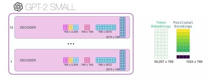
We have introduced the transformer module as thoroughly as possible. Now, you have basically mastered most of what happens inside the transformer language model. To recap, a new input vector will encounter the following weight matrices:
Moreover, each module has its own set of weights. On the other hand, this model has only one word embedding matrix and one positional encoding matrix:
If you want to know all the parameters in the model, here are detailed statistics:
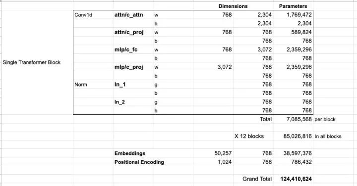
For some reason, the model has a total of 124 million parameters instead of 117 million. I am not sure why, but this seems to be the number in the released code (if this article has incorrect statistics, readers are welcome to point them out).
Part Three: Beyond Language Modeling
The transformer that only contains decoders continues to show promising applications beyond language modeling. In many applications, such models have achieved success, which can be described with visualization charts similar to the ones above. At the end of the article, let’s review some of these applications together.
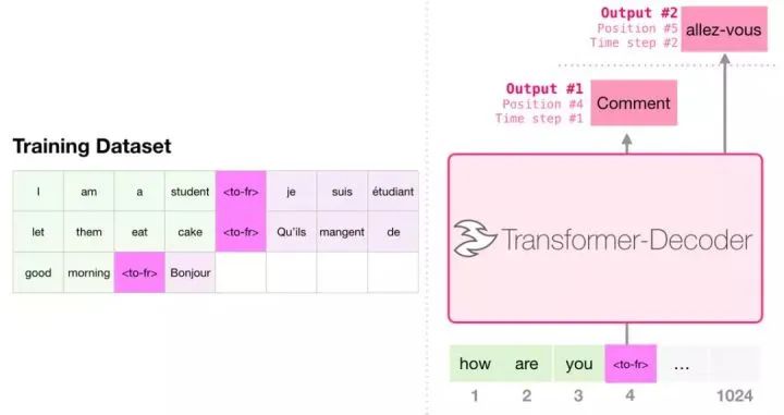
Machine Translation
When performing translation, the model does not need an encoder. The same task can be solved by a transformer that only has a decoder:
Automatic Summary Generation
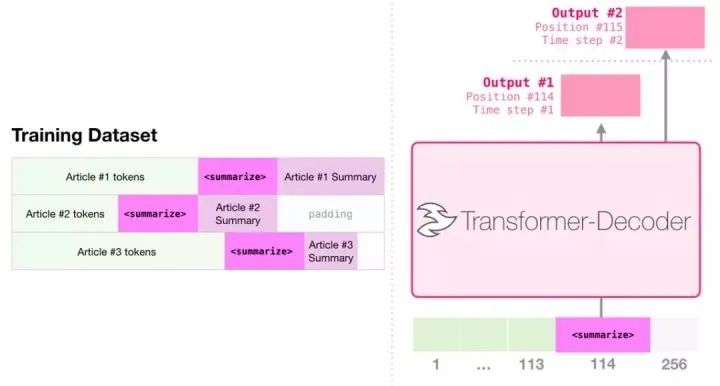
This is the first task for which a transformer containing only decoders was trained. That is, the model was trained to read Wikipedia articles (excluding the introductory parts before the table of contents) and then generate summaries. The actual introductory parts of the articles were used as labels in the training dataset:
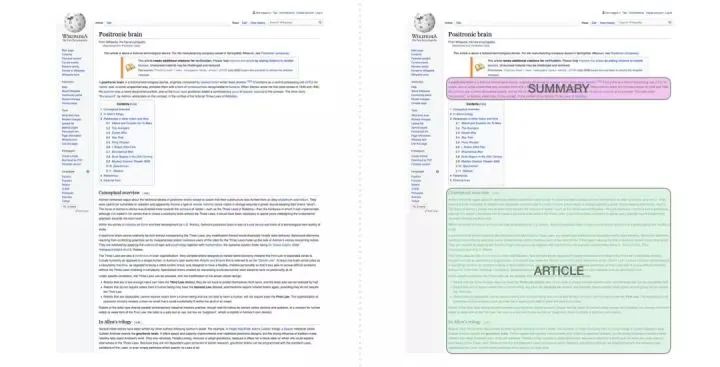
The model trained on Wikipedia articles was able to generate summaries of the articles:
Transfer Learning
In the paper “Sample Efficient Text Summarization Using a Single Pre-Trained Transformer” (arxiv.org/abs/1905.0883), a transformer containing only decoders was first pre-trained on language modeling tasks and then fine-tuned for summary generation tasks. The results showed that in cases with limited data, this approach achieved better results than the pre-trained encoder-decoder transformer.
The GPT-2 paper also demonstrated the summary generation effects obtained after pre-training the language modeling model.
Music Generation
The music transformer (magenta.tensorflow.org/) uses a transformer that only contains decoders (magenta.tensorflow.org/) to generate music with rich rhythms and dynamics. Similar to language modeling, “music modeling” allows the model to learn music in an unsupervised manner and then output samples (which we previously referred to as “random work”).
You might be curious about how music is represented in this context. Keep in mind that language modeling can be achieved through vector representations of characters, words, or parts of words (tokens). When dealing with a piece of music performance (temporarily using the piano as an example), we not only need to represent these notes but also the tempo—an indicator of the force with which the piano keys are pressed.
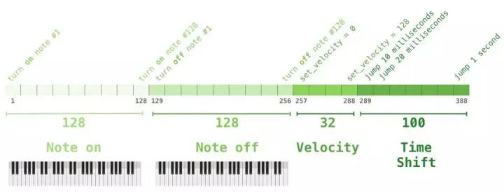
A performance can be represented as a series of one-hot vectors. A MIDI file can be converted into this format. The paper presents examples of input sequences in this format.
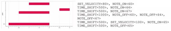
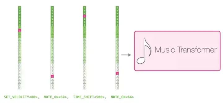
The one-hot vector representation of this input sequence is as follows:
I like the visualization charts used in the paper to demonstrate the self-attention mechanism in music transformers. I have added some annotations here:
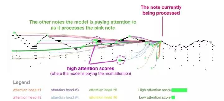
This piece features a recurring triangular contour. The current query vector is located at the back of a “peak”, focusing on the high notes on all previous peaks, all the way to the beginning of the piece. The diagram shows a query vector (the source of all attention lines) and the previous memory being processed (highlighted are the notes with higher softmax probabilities). The colors of the attention lines correspond to different attention heads, and the widths correspond to the weights of the softmax probabilities.
If you want to learn more about the representation of music notes, please watch the video below: youtube.com/watch?
Conclusion
Thus concludes our complete interpretation of GPT-2 and the analysis of its parent model (the transformer that only contains decoders). I hope readers can gain a better understanding of the self-attention mechanism through this article. After understanding how the transformer works internally, you will be more adept when encountering it next time.
Original address: jalammar.github.io/illu
Important! The Yizhen Natural Language Processing – Academic WeChat Group has been established
You can scan the QR code below to join the group for discussion,
Note: Please modify your remarks to [School/Company + Name + Direction] when adding.
For example – Harbin Institute of Technology + Zhang San + Dialogue System.
Account owner, please avoid business promotions. Thank you!

Recommended Reading:
【Long Article Explanation】From Transformer to BERT Model
Sai Er Translation | Understanding Transformer from Scratch
A picture is worth a thousand words! A step-by-step guide to building a Transformer with Python