
XGBoost is well-known as a powerful tool in data science competitions and is widely used in the industry. This article shares a collection of frequently asked interview questions about XGBoost that I have compiled over the years, hoping to deepen everyone’s understanding of XGBoost and, more importantly, to provide some assistance when seeking opportunities.
1. Brief Introduction to XGBoost
2. What Are the Differences Between XGBoost and GBDT?
-
Base Classifier: XGBoost’s base classifier not only supports CART decision trees but also supports linear classifiers. In this case, XGBoost is equivalent to logistic regression (for classification problems) or linear regression (for regression problems) with L1 and L2 regularization terms. -
Derivative Information: XGBoost performs a second-order Taylor expansion of the loss function, while GBDT only uses first-order derivative information. XGBoost also supports custom loss functions as long as the first and second derivatives are available. -
Regularization Terms: XGBoost’s objective function includes regularization terms, which act as pre-pruning, making the learned model less prone to overfitting. -
Column Sampling: XGBoost supports column sampling, similar to random forests, to prevent overfitting. -
Missing Value Handling: For each non-leaf node in the tree, XGBoost can automatically learn its default split direction. If a sample has a missing feature value, it will be assigned to the default branch. -
Parallelization: Note that this is not tree-level parallelism but feature-level parallelism. XGBoost pre-sorts each feature by feature value and stores them in a block structure, allowing multi-threaded parallel search for the best split points for each feature during node splitting, greatly improving training speed.
3. Why Does XGBoost Use Second-Order Taylor Expansion?
-
Precision: Compared to GBDT’s first-order Taylor expansion, XGBoost’s second-order Taylor expansion can more accurately approximate the true loss function.
-
Scalability: The loss function supports custom definitions as long as the new loss function is second-order differentiable.
4. Why Can XGBoost Train in Parallel?
-
XGBoost’s parallelism does not mean that each tree can be trained in parallel; XGBoost essentially still follows the boosting idea, where each tree must wait for the previous one to finish training before starting.
-
XGBoost’s parallelism refers to feature-level parallelism: before training, each feature is pre-sorted by feature value and stored in a block structure. When searching for feature split points later, this structure can be reused, and since features are stored in block structures, multi-threading can be used to compute the best split points for each block in parallel.
5. Why is XGBoost Fast?
-
Block Parallelism: Each feature is sorted by feature value and stored in a block structure before training, which can be reused when searching for feature split points, and supports parallel searching for each feature’s split points.
-
Candidate Split Points: Each feature uses a constant number of quantile points as candidate split points.
-
CPU Cache Hit Optimization: Using cache prefetching methods, each thread is allocated a continuous buffer to read the gradient information of samples in each block and store it in a continuous buffer.
-
Block Processing Optimization: Blocks are pre-loaded into memory; blocks are decompressed by columns; blocks are divided across different disks to improve throughput.
6. How Does XGBoost Prevent Overfitting?
-
Adding Regularization Terms to the Objective Function: L2 regularization on the number of leaf nodes and the weights of leaf nodes. -
Column Sampling: During training, only a portion of features is used (the remaining block can be ignored). -
Subsampling: Not all samples are used in each iteration, making the algorithm more conservative. -
Shrinkage: Also known as learning rate or step size, to leave more learning space for subsequent training.
7. How Does XGBoost Handle Missing Values?
One advantage of the XGBoost model is that it allows features to have missing values. The approach to handling missing values is as follows:
-
When searching for the best split point on feature k, samples with missing values in that feature are not traversed; only the corresponding feature values of non-missing samples are traversed, reducing the time cost of finding split points for sparse discrete features.
-
In terms of logical implementation, to ensure completeness, samples with missing feature values are assigned to both left and right leaf nodes, and both scenarios are calculated. The direction with the highest gain after splitting (left or right) is chosen as the default direction for samples with missing feature values during prediction.
-
If there are no missing values during training but missing values appear during prediction, the split direction for missing values will automatically be assigned to the right child node.
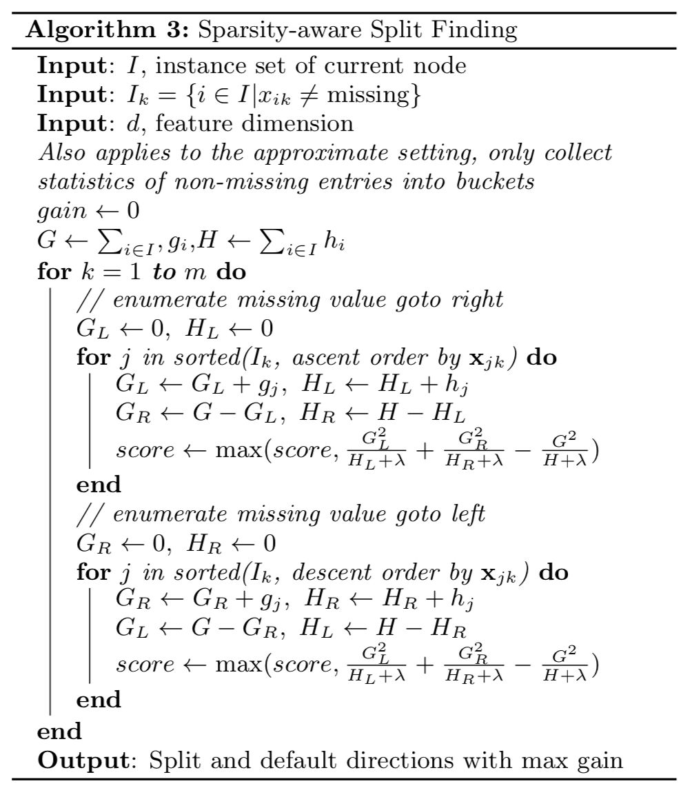
Pseudocode for handling missing values during find_split
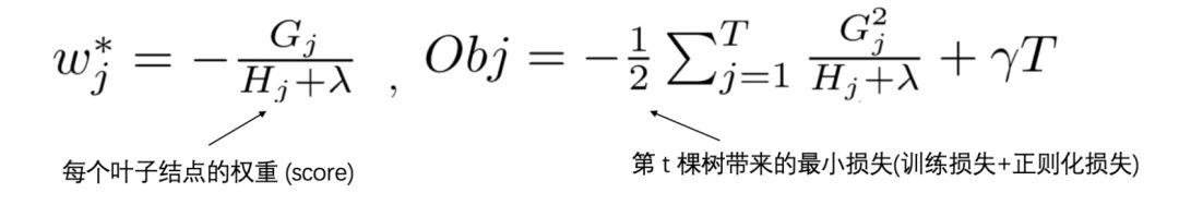
8. How Are Leaf Node Weights Calculated in XGBoost?
The final derived form of the XGBoost objective function is as follows:
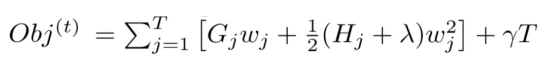
The specific formula is as follows:
9. Stopping Conditions for Tree Growth in XGBoost
-
When the gain from a new split is less than 0, the current split is abandoned. This is a trade-off between training loss and model complexity.
-
When the tree reaches its maximum depth, tree building stops as deeper trees are prone to overfitting; thus, a hyperparameter max_depth needs to be set.
-
After introducing a split, the sample weights of the newly generated left and right leaf nodes are recalculated. If the sample weight of any leaf node is below a certain threshold, that split will also be abandoned. This involves a hyperparameter: minimum sample weight sum, which indicates that if a leaf node contains too few samples, the split will also be abandoned to prevent overly fine splits.
10. Differences Between RF and GBDT
Similarities:
-
Both consist of multiple trees, and the final result is determined by the ensemble of these trees.
Differences:
-
Ensemble Learning: RF follows the bagging approach, while GBDT follows the boosting approach. -
Bias-Variance Trade-off: RF continuously reduces model variance, while GBDT continuously reduces model bias. -
Training Samples: RF samples from the entire training set with replacement for each iteration, while GBDT uses all samples each time. -
Parallelism: RF trees can be generated in parallel, while GBDT trees can only be generated sequentially (waiting for the previous tree to be fully generated). -
Final Result: RF ultimately uses majority voting among multiple trees (averaging for regression), while GBDT uses weighted fusion. -
Data Sensitivity: RF is insensitive to outliers, while GBDT is sensitive to outliers. -
Generalization Ability: RF is less prone to overfitting, while GBDT is more prone to overfitting.
11. How Does XGBoost Handle Imbalanced Data?
For imbalanced datasets, such as user purchase behaviors, which are extremely imbalanced, this significantly impacts XGBoost training. XGBoost has two built-in methods to address this:
First, if you care about AUC and use it to evaluate model performance, you can balance the weights of positive and negative samples by setting scale_pos_weight. For example, when the positive to negative sample ratio is 1:10, scale_pos_weight can be set to 10;
Second, if you care about probability (the rationality of predicted scores), you should not rebalance the dataset (as it would distort the true distribution of the data). Instead, set max_delta_step to a finite number to help convergence (effective when the base model is LR).
The original statement is as follows:
For common cases such as ads clickthrough log, the dataset is extremely imbalanced. This can affect the training of xgboost model, and there are two ways to improve it. If you care only about the ranking order (AUC) of your prediction Balance the positive and negative weights, via scale_pos_weight Use AUC for evaluation If you care about predicting the right probability In such a case, you cannot re-balance the dataset In such a case, set parameter max_delta_step to a finite number (say 1) will help convergenceSo, how does the source code utilize scale_pos_weight to balance samples? Is it adjusting weights or oversampling? Please see the source code:
if (info.labels[i] == 1.0f) w *= param_.scale_pos_weightIt can be seen that the weight of minority samples is increased.
In addition, oversampling, undersampling, SMOTE algorithms, or custom cost functions can also be used to address the imbalance between positive and negative samples.
12. Compare LR and GBDT, and Discuss Situations Where GBDT Is Inferior to LR
First, let’s discuss the differences between LR and GBDT:
-
LR is a linear model with strong interpretability, easy to parallelize, but has limited learning ability and requires extensive manual feature engineering. -
GBDT is a nonlinear model with a natural advantage in feature combination and strong feature expression ability, but trees cannot be trained in parallel, and tree models are prone to overfitting.
In scenarios with high-dimensional sparse features, LR generally performs better than GBDT. The reason is as follows:
Consider an example:
Assuming a binary classification problem with labels 0 and 1, and 100-dimensional features, if there are 10,000 samples but only 10 positive samples, and all the feature values of feature f1 for those 10 positive samples are 1, while the remaining 9,990 samples have a feature f1 value of 0 (this situation is common with high-dimensional sparsity).
We know that in this case, tree models can easily optimize a tree using feature f1 as an important splitting node because this node can perfectly separate the training data. However, during testing, it may perform poorly because the feature f1 just coincidentally fitted this pattern with y, which is what we call overfitting.
In this case, if we use LR, we would think it might also exhibit similar overfitting: y = W1*f1 + Wi*fi+… where W1 is particularly large to fit these 10 samples. Why does the tree model overfit more severely in this case?
Upon reflection, we find that modern models generally include regularization terms, and the regularization term for linear models like LR penalizes weights, meaning that if W1 becomes too large, the penalty will be significant, further compressing W1’s value to prevent it from becoming too large. However, tree models are different; their penalty terms are typically based on the number of leaf nodes and depth, and we know that in the above case, the tree only needs one node to perfectly separate the 9,990 and 10 samples, resulting in an extremely small penalty term.
This is why linear models with regularization are less likely to overfit sparse features compared to nonlinear models.
13. How Does XGBoost Prune Trees?
-
By adding a regularization term to the objective function: using the number of leaf nodes and the square of the L2 norm of leaf node weights to control tree complexity.
-
During node splitting, a threshold is defined. If the gain of the objective function after splitting is below this threshold, the split is not made.
-
After introducing a split, the sample weights of the newly generated left and right leaf nodes are recalculated. If the sample weight of any leaf node is below a certain threshold (minimum sample weight sum), that split will also be abandoned.
-
XGBoost first builds trees from top to bottom until the maximum depth, then checks from bottom to top for nodes that do not meet the splitting conditions to perform pruning.
14. How Does XGBoost Select the Best Split Points?
15. How Is the Scalability of XGBoost Reflected?
-
Scalability of Base Classifiers: Weak classifiers can support CART decision trees as well as LR and Linear. -
Scalability of Objective Functions: Supports custom loss functions as long as they are first and second order differentiable. This feature is due to the second-order Taylor expansion, resulting in a general form of the objective function. -
Scalability of Learning Methods: The block structure supports parallelization and out-of-core computation.
16. How Does XGBoost Evaluate Feature Importance?
We use three methods to assess the importance of features in the XGBoost model:
Official documentation: (1) weight - the number of times a feature is used to split the data across all trees. (2) gain - the average gain of the feature when it is used in trees. (3) cover - the average coverage of the feature when it is used in trees.-
Weight: The total number of times this feature is used to split samples across all trees.
-
Gain: The average gain produced by this feature in all trees where it appears.
-
Cover: The average coverage of this feature across all trees where it appears.
Note: Coverage here refers to the number of samples influenced by a feature when used as a split point, i.e., how many samples are split into two child nodes by this feature.
17. General Steps for Tuning XGBoost Parameters
First, some basic variables need to be initialized, for example:
-
max_depth = 5
-
min_child_weight = 1
-
gamma = 0
-
subsample, colsample_bytree = 0.8
-
scale_pos_weight = 1
We adjust these two parameters because they have a significant impact on output results. We first set these parameters to larger numbers and then iteratively refine them to narrow down the range.
Max depth, the maximum depth of each subtree, check from range (3,10,2).
Min child weight, the weight threshold for child nodes, check from range (1,6,2).
If the sum of weights of all child nodes after a split exceeds this threshold, the leaf node can be split.
min_split_loss, check from 0.1 to 0.5, indicating the threshold for the reduction in the loss function after making a split for a leaf node.-
If greater than this threshold, the leaf node is worth continuing to split.
-
If less than this threshold, the leaf node is not worth continuing to split.
Subsample refers to the sampling ratio of the training data.
Colsample by tree refers to the sampling ratio of features.
Both check from 0.6 to 0.9.
Alpha is the L1 regularization coefficient, try 1e-5, 1e-2, 0.1, 1, 100.
Lambda is the L2 regularization coefficient.
18. How to Solve Overfitting in XGBoost Models?
<span>max_depth,min_child_weight,gamma</span> and other parameters.<span>subsample,colsample_bytree</span>learning rate while increasing estimator parameters can also help.19. Why is XGBoost Less Sensitive to Missing Values Compared to Some Models?
For features with missing values, common solutions include:
-
For categorical variables: fill in with the most frequently occurring feature value;
-
For continuous variables: fill in with the median or mean;
-
When the data volume is small, prefer naive Bayes. -
When the data volume is moderate or large, use tree models, preferably XGBoost. -
When the data volume is very large, neural networks can also be used. -
Avoid using models related to distance measurement, such as KNN and SVM.
20. Differences Between XGBoost and LightGBM
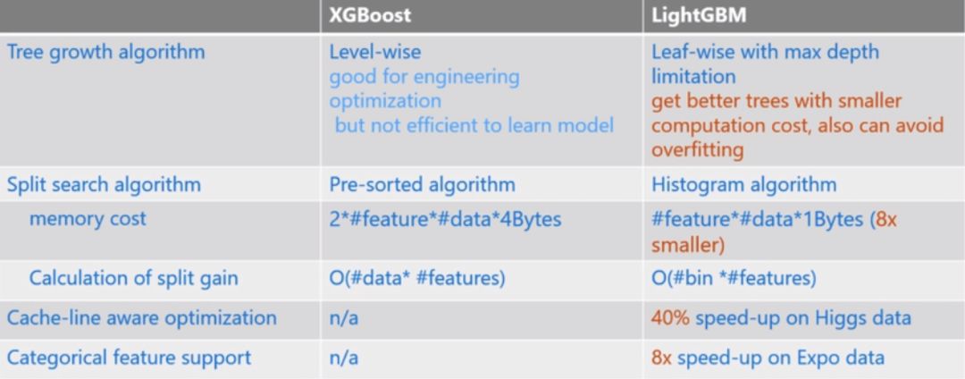
level-wise splitting strategy, while LGB uses a leaf-wise splitting strategy. XGB indiscriminately splits all nodes at each level, but some nodes may have very small gains, which do not significantly impact the results, leading to unnecessary overhead. Leaf-wise selects the node with the highest splitting gain among all leaf nodes, but it can easily lead to overfitting, so maximum depth needs to be limited.-
Reduces memory usage. For example, when discretized into 256 bins, only 8 bits are needed to store which bin a sample is mapped to (this bin can be considered as the transformed feature). Compared to the pre-sorted exact greedy algorithm (which uses int_32 to store indices + float_32 to store feature values), this can save 7/8 of the space. -
Improves computational efficiency. The exact greedy algorithm requires traversing all data for each feature and calculating gains, with a complexity of 𝑂(#𝑓𝑒𝑎𝑡𝑢𝑟𝑒×#𝑑𝑎𝑡𝑎). The histogram algorithm, after creating the histogram, only needs to traverse the histogram for each feature, with a complexity of 𝑂(#𝑓𝑒𝑎𝑡𝑢𝑟𝑒×#𝑏𝑖𝑛𝑠). -
LGB can also use histogram difference acceleration; a node’s histogram can be obtained by subtracting the sibling node’s histogram from the parent node’s histogram, thus speeding up calculations.
However, XGBoost’s approximate histogram algorithm is also similar to LightGBM’s histogram algorithm. Why is XGBoost’s approximate algorithm still much slower than LightGBM? XGBoost dynamically constructs histograms at each level because its histogram algorithm does not target a specific feature; instead, all features share a histogram (with each sample’s weight being the second derivative). Therefore, histograms need to be reconstructed at each level, while LightGBM has a histogram for each feature, so constructing a histogram once is sufficient.
-
Feature Parallelism: LightGBM’s feature parallelism requires each worker to have a complete dataset, but each worker only finds the best split points on a subset of features. Workers need to communicate to determine the best split point, which is then globally broadcasted for each worker to perform the split. The main difference between XGBoost’s feature parallelism and LightGBM’s is that in XGBoost, each worker only has a portion of the column data, meaning vertical splits, while each worker finds local best split points, communicates with each other, and then performs node splitting on the worker with the best split point. This difference results in significantly lower communication costs in LightGBM, requiring only communication of a feature split point, while XGBoost broadcasts sample indices for splitting.
Data Parallelism: When the data volume is large and the features are relatively few, data parallel strategies can be adopted. In LightGBM, data is first split horizontally, and each worker builds local histograms, which are then merged into a global histogram. Using histogram subtraction, the sample indices for nodes with fewer samples are calculated, and the other child node’s sample indices are directly obtained, reducing communication costs between workers by half, as only the sample indices for the node with fewer samples need to be communicated. In XGBoost, data is also split horizontally, and each worker builds local histograms, but when splitting nodes based on the global histogram, sample indices for child nodes must be calculated separately, leading to slow efficiency and increased communication volume between workers.
Voting Parallelism (LightGBM): When both the data volume and dimensions are large, voting parallelism can be selected. This method is an improvement over data parallelism. The cost of merging histograms in data parallelism is relatively high, especially when feature dimensions are large. The general idea is that each worker first finds some excellent local features and then conducts a global vote to select the top features for histogram merging, seeking the global optimal split point.
References:
1. https://blog.csdn.net/u010665216/article/details/78532619
2. https://blog.csdn.net/jamexfx/article/details/93780308