Building a 3D-CNN in TensorFlow

Click on the above “3D Vision Workshop“, select “Star”

Delivering valuable content promptly

Author | Pan Duoduo

Source | Deep Learning and Computer Vision

Introduction to 3D-CNN

The MNIST dataset classification is considered the hello world program in the field of computer vision. The MNIST dataset helps beginners understand the concept and implementation of Convolutional Neural Networks (CNN).

MNIST dataset: https://www.analyticsvidhya.com/blog/2022/04/binary-classification-on-skin-cancer-dataset-using-dl/

Many people think of an image as just an ordinary matrix, but that is not the case. Images have what is called spatial information. Consider the following 3X3 matrix.

[a b c

d e f

g h i]

In a regular matrix, the values in the matrix will be independent of each other. Adjacent values do not carry any relationship or information about specific fields in the matrix. For example, the value replacing “e” in the matrix has no relation to values appearing elsewhere (like “a”, “b”, etc.). This is not the case with images.

In an image, each position in the matrix represents a pixel in the image, and the value of each position represents the value of that pixel. Pixel values can range from [0-255] in an 8-bit image. Each pixel has some relationship with its neighboring pixels. The neighborhood of any pixel is a set of pixels surrounding it. There are three ways to represent the neighborhood of any pixel, called N-4, ND, and N-8. Let’s delve into them in detail.

1. N-4: It represents the pixels located above, below, to the right, and to the left of the reference pixel. For pixel “e”, N-4 contains “b”, “f”, “h”, and “d”.
2. ND: It represents the pixels accessible from the diagonal of the reference pixel. For pixel “e”, ND contains “a”, “c”, “i”, and “g”.
3. N-8: It represents all pixels surrounding it. It includes both N-4 and ND pixels. For pixel “e”, N-8 contains “a”, “b”, “c”, “d”, “f”, “g”, “h”, and “i”.

N-4, N-8, and ND pixels help extract information about pixels. For example, these parameters can be used to classify pixels as boundary or internal or external pixels. This is the peculiarity of images. Artificial Neural Networks (ANN) receive input in the form of one-dimensional arrays. Images always exist in a 2D array with one or more channels. When the image array is converted to a one-dimensional array, it loses spatial information, so the ANN cannot capture this information and performs poorly on image datasets. And this is where CNN excels.

CNN accepts 2D arrays as input and performs convolution operations using masks (or filters or kernels) to extract these features. The process called pooling reduces the number of extracted features and lowers computational complexity. After completing these operations, we convert the extracted features into a 1D array and provide it to the neural network layer for learning and classification.

This article aims to extend the concept of performing convolution operations on 3D data. We will build a 3D CNN that will perform classification on the 3D MNIST dataset.

Download the dataset from here: https://www.kaggle.com/datasets/daavoo/3d-mnist

Dataset Overview

We will use the fulldatasetvectors.h5 file in the dataset. This file contains 4096-D vectors obtained from voxelization (x:16, y:16, z:16) of all 3D point clouds. The file contains 10,000 training samples and 2,000 testing samples. The dataset also has available point cloud data.

Detailed information about the dataset can be found here: https://www.kaggle.com/datasets/daavoo/3d-mnist. Feel free to read more about the dataset before proceeding.

Importing Modules

Since the data is stored in h5 format, we will use the h5py module to load the dataset from the fulldatasetvectors file. TensorFlow and Keras will be used to build and train the 3D-CNN. The to_categorical function helps perform one-hot encoding on the target variable. We will also use the early stopping callback to stop training and prevent the model from overfitting.

import numpy as np 
import h5py
from tensorflow.keras.utils import to_categorical
from tensorflow.keras import layers
from tensorflow.keras.models import Sequential
from tensorflow.keras.initializers import Constant
from tensorflow.keras.optimizers import Adam
from tensorflow.keras.callbacks import EarlyStopping

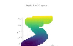
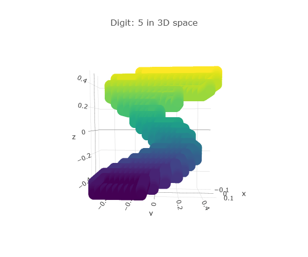
Loading the Dataset

As mentioned earlier, we will use the h5py module to load data from the fulldatasetvectors.h5 file.

Using h5py.File(‘../input/3d-mnist/full_dataset_vectors.h5’, ‘r’) as dataset:

xtrain, xtest = dataset["X_train"][:], dataset["X_test"][:]
ytrain, ytest = dataset["y_train"][:], dataset["y_test"][:]
xtrain = np.array(xtrain)
xtest = np.array(xtest)
print('train shape:', xtrain.shape)
print('test shape:', xtest.shape)
xtrain = xtrain.reshape(xtrain.shape[0], 16, 16, 16, 1)
extest = xtest.reshape(xtest.shape[0], 16, 16, 16, 1)
ytrain, ytest = to_categorical(ytrain, 10), to_categorical(ytest, 10)

We can see that the training data has 10,000 samples, while the testing data has 2,000 samples, each sample containing 4,096 features.

train shape: (10000, 4096)
test shape: (2000, 4096)

Building the 3D-CNN

A 3D-CNN, like any regular CNN, has two parts – a feature extractor and an ANN classifier, and operates in the same way.

Unlike a regular CNN, a 3D-CNN performs 3D convolutions instead of 2D convolutions. We will use Keras’s Sequential API to build the 3D CNN. The first two layers will be 3D convolution layers with 32 filters and ReLU as the activation function, followed by a max pooling layer for dimensionality reduction. These layers also add a bias term with a value of 0.01. By default, the bias value is set to 0.

Again using the same set of layers but with 64 filters. Then a dropout layer and a flatten layer. The flatten layer helps reshape the features into a one-dimensional array that can be processed by the artificial neural network, i.e., the dense layer. The ANN part consists of 2 layers with 256 and 128 neurons, respectively, using ReLU as the activation function. The output layer has 10 neurons since there are 10 different categories or labels in the dataset.

model = Sequential()
model.add(layers.Conv3D(32,(3,3,3),activation='relu',input_shape=(16,16,16,1),bias_initializer=Constant(0.01)))
model.add(layers.Conv3D(32,(3,3,3),activation='relu',bias_initializer=Constant(0.01)))
model.add(layers.MaxPooling3D((2,2,2)))
model.add(layers.Conv3D(64,(3,3,3),activation='relu'))
model.add(layers.Conv3D(64,(2,2,2),activation='relu'))
model.add(layers.MaxPooling3D((2,2,2)))
model.add(layers.Dropout(0.6))
model.add(layers.Flatten())
model.add(layers.Dense(256,'relu'))
model.add(layers.Dropout(0.7))
model.add(layers.Dense(128,'relu'))
model.add(layers.Dropout(0.5))
model.add(layers.Dense(10,'softmax'))
model.summary()

This is the architecture of the 3D-CNN.

Model: "sequential_2"
_________________________________________________________________
Layer (type)                 Output Shape              Param #   
=================================================================
conv3d_5 (Conv3D)            (None, 14, 14, 14, 32)    896       
_________________________________________________________________
conv3d_6 (Conv3D)            (None, 12, 12, 12, 32)    27680     
_________________________________________________________________
max_pooling3d_2 (MaxPooling3 (None, 6, 6, 6, 32)       0         
_________________________________________________________________
conv3d_7 (Conv3D)            (None, 4, 4, 4, 64)       55360     
_________________________________________________________________
conv3d_8 (Conv3D)            (None, 3, 3, 3, 64)       32832     
_________________________________________________________________
max_pooling3d_3 (MaxPooling3 (None, 1, 1, 1, 64)       0         
_________________________________________________________________
dropout_4 (Dropout)          (None, 1, 1, 1, 64)       0         
_________________________________________________________________
flatten_1 (Flatten)          (None, 64)                0         
_________________________________________________________________
dense_3 (Dense)              (None, 256)               16640     
_________________________________________________________________
dropout_5 (Dropout)          (None, 256)               0         
_________________________________________________________________
dense_4 (Dense)              (None, 128)               32896     
_________________________________________________________________
dropout_6 (Dropout)          (None, 128)               0         
_________________________________________________________________
dense_5 (Dense)              (None, 10)                1290      
=================================================================
Total params: 167,594
Trainable params: 167,594
Non-trainable params: 0

Training the 3D-CNN

We will use Adam as the optimizer. Categorical cross-entropy will be used as the loss function for training the model since it is a multi-class classification. Accuracy will be used as the loss metric for training.

As mentioned earlier, the EarlyStopping callback will be used during model training and dropout layers. Once any parameter (such as loss or accuracy) does not improve for a certain number of periods, the EarlyStopping callback helps stop the training process, which in turn helps prevent the model from overfitting.

Dropout helps prevent the model from overfitting by randomly turning off some neurons during training and encouraging the model to learn rather than memorize. The dropout value should not be too high, or it may lead to underfitting, which is not ideal.

model.compile(Adam(0.001),'categorical_crossentropy',['accuracy'])
model.fit(xtrain,ytrain,epochs=200,batch_size=32,verbose=1,validation_data=(xtest,ytest),callbacks=[EarlyStopping(patience=15)])

These are some epochs for training the 3D-CNN.

Epoch 1/200
313/313 [==============================] - 39s 123ms/step - loss: 2.2782 - accuracy: 0.1237 - val_loss: 2.1293 - val_accuracy: 0.2235
Epoch 2/200
313/313 [==============================] - 39s 124ms/step - loss: 2.0718 - accuracy: 0.2480 - val_loss: 1.8067 - val_accuracy: 0.3395
Epoch 3/200
313/313 [==============================] - 39s 125ms/step - loss: 1.8384 - accuracy: 0.3382 - val_loss: 1.5670 - val_accuracy: 0.4260
...
...
Epoch 87/200
313/313 [==============================] - 39s 123ms/step - loss: 0.7541 - accuracy: 0.7327 - val_loss: 0.9970 - val_accuracy: 0.7061

Testing the 3D-CNN

The 3D-CNN achieved 73.3% accuracy on the training data and 70.6% accuracy on the testing data. Due to the very small and unbalanced dataset, the accuracy may be slightly low.

_, acc = model.evaluate(xtrain, ytrain)
print('training accuracy:', str(round(acc*100, 2))+'%')
_, acc = model.evaluate(xtest, ytest)
print('testing accuracy:', str(round(acc*100, 2))+'%')

313/313 [==============================] - 11s 34ms/step - loss: 0.7541 - accuracy: 0.7327
training accuracy: 73.27%
63/63 [==============================] - 2s 34ms/step - loss: 0.9970 - accuracy: 0.7060
testing accuracy: 70.61%

Conclusion

In conclusion, this article covers the following topics:

• The neighborhoods of pixels in images
• Why ANN performs poorly on image datasets
• The differences between CNN and ANN
• How CNN works
• Building and training a 3D-CNN in TensorFlow

To further continue this project, one could try creating a new custom 3D dataset from the MNIST dataset by projecting pixel values onto another axis. The x-axis and y-axis will remain the same as in any image, but the pixel values will be projected onto the z-axis. This transformation from 2D data to 3D data can be applied after performing image augmentation so that we have a balanced and general dataset for training the 3D-CNN and achieving better accuracy.

This article is for academic sharing only. If there is any infringement, please contact for deletion.

Download and learn valuable content

Reply in the background:BarcelonaAutonomous University courseware, to download the exquisite courseware of 3D Vision accumulated by foreign universities over the years

Reply in the background:Computer Vision books, to download classic books in the field of 3D vision pdf

Reply in the background:3D Vision course, to learn exquisite courses in the field of 3D vision

Official website of the 3D Vision Workshop exquisite course:3dcver.com

1. Multi-sensor data fusion technology for autonomous driving

2. Full-stack learning path for 3D point cloud target detection in the field of autonomous driving! (Single-modal + multi-modal/data + code) 3. Thoroughly understand visual 3D reconstruction: principle analysis, code explanation, and optimization improvement 4. The first industrial-level practical point cloud processing course in China 5. Laser-vision-IMU-GPS fusion SLAM algorithm sorting and code explanation 6. Thoroughly understand visual-inertial SLAM: based on VINS-Fusion officially launched 7. Thoroughly understand 3D laser SLAM based on the LOAM framework: from source code analysis to algorithm optimization

9. Build a structured light 3D reconstruction system from scratch [theory + source code + practice]

10. Monocular depth estimation methods: algorithm sorting and code implementation

11. Practical deployment of deep learning models in autonomous driving

12. Camera models and calibration (monocular + binocular + fisheye)

13.Heavyweight! Quadrotor: algorithms and practice

14.ROS2 from entry to mastery: theory and practice

15. The first 3D defect detection tutorial in China: theory, source code, and practice

Heavyweight!3DCVer-Academic paper writing submission WeChat group has been established

Scan to add the assistant’s WeChat, you can apply to join the 3D Vision Workshop – Academic paper writing and submission WeChat group, aimed at exchanging writing and submission matters for top conferences, top journals, SCI, EI, etc.

At the same time, you can also apply to join our subdivided direction group chat, currently mainly including3D Vision、CV&Deep Learning、SLAM、3D Reconstruction、Point Cloud Post-processing、Autonomous Driving, Multi-sensor Fusion, CV Entry, 3D Measurement, VR/AR, 3D Face Recognition, Medical Imaging, Defect Detection, Person Re-identification, Object Tracking, Visual Product Implementation, Visual Competitions, License Plate Recognition, Hardware Selection, Academic Exchange, Job Exchange, ORB-SLAM series source code exchange, Depth Estimation and other WeChat groups.

Please be sure to note: Research direction + School/Company + Nickname, for example: “3D Vision + Shanghai Jiao Tong University + Jingjing”. Please follow the format to be quickly approved and invited into the group. Original submissions should also contact us.

▲ Long press to add WeChat group or submit

▲ Long press to follow the public account

3D Vision from Entry to Mastery Knowledge Planet: Targeting the 3D Vision field video courses (3D Reconstruction series、3D Point Cloud series、Structured Light series、Hand-Eye Calibration、Camera Calibration、Laser/Vision SLAM, Autonomous Driving, etc.),Knowledge point summary, entry and advanced learning routes, latest paper sharing, Q&A Five aspects for in-depth cultivation, with various algorithm engineers from large companies providing technical guidance. Meanwhile, the planet will cooperate with well-known enterprises to release 3D vision-related algorithm development positions and project docking information, creating a fan gathering area that integrates technology and employment, with nearly 5,000 planet members working together to create a better AI world.

Learn core technologies of 3D Vision, scan to view the introduction, unconditional refund within 3 days

There are high-quality tutorial materials, Q&A to help you efficiently solve problems

If you find it useful, please give a thumbs up and watch~