Breaking the BERT Ceiling: 11 Techniques to Boost NLP Classification SOTA

Source | Xixiaoyao’s Cute Selling House

At this point in 2020, our focus on NLP classification tasks is no longer about how to construct models or being fixated on what classification models look like. Just like the current focus in the CV field, we should pay more attention to how to utilize machine learning ideas to better address issues in NLP classification tasks such as low time consumption, small samples, robustness, imbalance, testing and verification, incremental learning, and long texts.

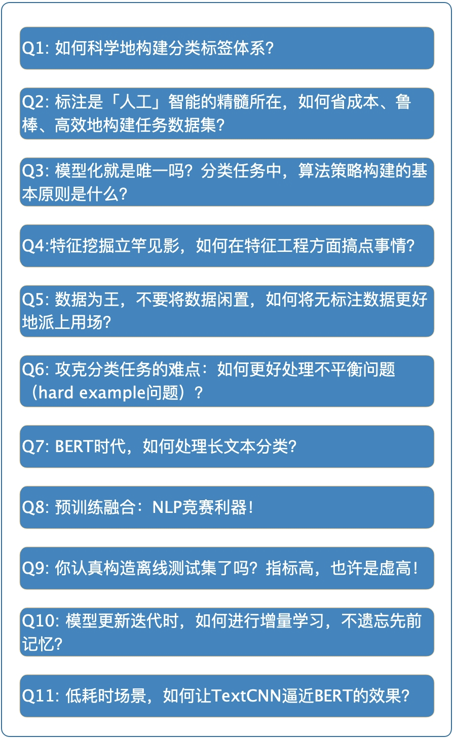
This article discusses the following questions in a Q&A format:

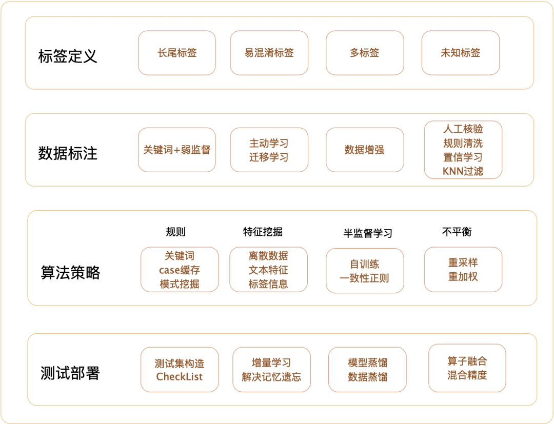
NLP classification tasks are familiar to every NLPer, as they play a crucial role in the entire NLP business. More sub-tasks in various fields often convert into classification tasks, such as news classification, sentiment recognition, intent recognition, relation classification, event type judgment, and so on. Constructing a complete NLP classification task mainly includes four parts: label definition, data construction, algorithm strategy, and testing deployment. The organization structure of this article is shown in the figure below.

Statement: The views in this article represent the author’s personal position. Blindly copying carries risks~

Q1: How to Scientifically Construct a Classification Label System?

The definition of classification labels is crucial. When faced with complex label issues, the key point is to closely align with the business and set it together with experts, rather than relying on brute force to solve it. Here are some label definition methods that I have been involved in:

1. Long-tail labels: Some classification labels naturally have very few samples, which can be set as “others”, and then further processed separately at the next level.
2. Confusable labels: Some labels have samples that are difficult to distinguish. First, consider whether these labels can be merged directly; if not, unify these labels first, and then process them with rules at the next level.
3. Multi-label: In some scenarios, label settings may reach hundreds, and a multi-level label system can be set up for processing. For example, first construct a large category of labels, then build subcategories; or set multiple binary classifications, suitable for scenarios where label classifications are relatively independent and often need to be added or modified, allowing for independence and ease of maintenance.
4. Unknown labels: During business cold starts, if it is unclear which labels are appropriate, one can attempt to preliminarily divide labels using text clustering methods, supplemented by expert involvement in setting them, which is also a cyclical iterative process.

For the above “long-tail labels” and “confusable labels”, it is also possible to optimize at the model level, which often involves issues of sample imbalance and hard example processing, which we will elaborate on later.

Q2: Labeling is the Essence of “Artificial” Intelligence; How to Build a Task Dataset Cost-Effectively, Robustly, and Efficiently?

Once the label definitions are set, the next step is to construct the classification task dataset. Dataset construction is an important part of daily work. It must be cost-effective, robust, and efficient. The main process of constructing a dataset includes the following four steps:

1. Construct the initial dataset: Produce about 100 samples for each label. Specific measures can include keyword matching and other rule-based methods, followed by manual checks.
2. “Active learning + Transfer learning” to reduce labeling scale: 1) Active learning aims to mine high-value samples: that is, through constructing a small number of samples that can meet indicator requirements. Based on the initially constructed dataset, a base model can be trained, and then some samples with high uncertainty (maximum entropy) + high representativeness (non-outliers) can be selected for manual labeling. 2) Transfer learning reduces dependence on data: The success of pre-trained language models in transfer learning allows for fine-tuning with fewer labeled samples to achieve target indicators.
3. Expand labeling scale; data augmentation is crucial: In scenarios with a small labeling scale, data can be expanded through text augmentation techniques, leveraging data leverage. In the article “Exploring the Dilemma of Few Samples in NLP”, we explored relevant text augmentation techniques in detail.
4. Clean data noise to make the model more robust: Strict quality control is required for labeling quality. In addition to manual checks, the following automated methods can be used to build a denoising system: 1) Manual rule cleaning: Configure black and white lists containing keyword information for strict rule cleaning. 2) Cross-validation: Cross-validate the training set and remove or manually correct samples with inconsistent labels. 3) Confidence learning: Essentially a further extension of cross-validation, constructing a confidence confusion matrix and introducing a ranking mechanism to filter noise samples. The article “Don’t Let Data Trap You! Use Confidence Learning to Identify Incorrect Labels” provides a detailed introduction. 4) Deep KNN filtering: The nearest neighbor metric in KNN makes it more effective in robust learning. The article “Deep k-NN for Noisy Labels” shows that even if deep models are trained on noisy data, adapting the intermediate layer representations to KNN for noise sample filtering significantly improves performance.

In constructing the dataset, in addition to the above four steps, attention must be paid to details and principle issues:

• For few-shot problems, do not blindly pursue the implementation of cutting-edge algorithms. Many times, we want to rely on a certain method to universally solve low-resource issues, but in reality, the time spent on strategic research is often too long, and the indicator gains are not as quick as direct manual labeling of data. I have found that for the vast majority of few-shot problems, necessary manual labeling cannot be avoided; combining multiple strategies with “planned and strategic” manual labeling may be the best way to solve few-shot issues.
• Is intelligent labeling a false proposition? The essence of intelligent labeling is efficiency, but active learning is often not efficient. Active learning requires multiple queries to the expert system for labeling. Therefore, when using active learning methods, it is essential to reduce not only the labeling scale but also the number of queries. In practice, we can prioritize actively querying category labels with significant indicator gains based on empirical formulas. We can also estimate the amount of data needed to meet the gain target based on empirical formulas. It is acceptable to query once and satisfy the requirements; marking a bit more is fine. Whether the so-called “intelligent labeling system” is genuinely intelligent, I feel that it still cannot completely detach from human intervention.
• Pre-trained models must have domain relevance; do not stop pre-training! When the labeled data for the task is scarce and the domain is less related to the initial pre-training corpus, do not stop domain pre-training!

I have provided a brief summary of the experimental results for the above strategies, as shown in the figure below: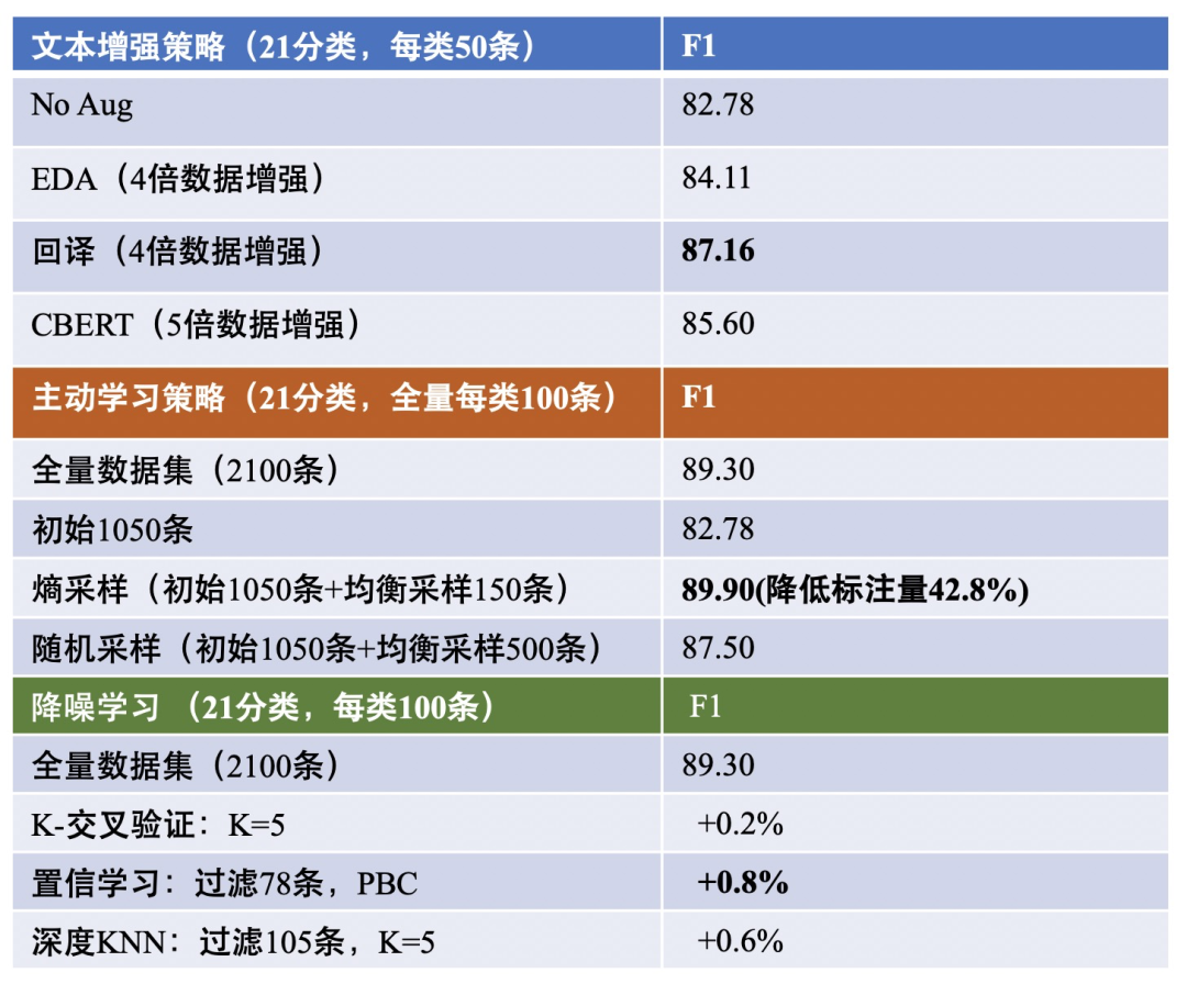

Q3: Is Modeling the Only Way? What Are the Basic Principles for Building Algorithm Strategies in Classification Tasks?

Algorithm strategies mainly include rule mining and modeling methods. The basic principles should be:

1. Rule fallback: High-frequency cases and hard cases should first enter the rule module to prevent the handling of important cases from being insufficiently robust due to model updates and iterations. Rule mining mainly includes important case caching, pattern mining, keyword + rule settings, etc. Additionally, rules can also follow the classification model for fallback processing.
2. Model generalization: Modeling methods are suitable for handling cases that cannot hit rules and should possess generalization ability. Another processing logic is: if a case hits a rule but the model gives a very low confidence level for the rule’s prediction result (meaning the model believes another category’s confidence is higher), we can choose to trust the model and take its output as the standard.

However, whether for rules or models, handling long-tail issues is quite tricky, but we can enhance the ability to handle long-tail cases as much as possible through some means (specifically introduced in Q6).

Q4: Feature extraction is immediate; how to make an impact in feature engineering?

For NLP classification tasks, especially in vertical domain classification tasks, if we can better extract features at the business feature level, the indicator gains can be immediate~

In terms of feature engineering, I mainly provide three techniques:

• Discrete data mining
• Construct high-dimensional sparse features from keywords: Similar to structured data mining (like wide&deep in CTR), for example, mining text content based on a keyword list, constructing high-dimensional sparse features, and feeding them into xDeepFM^[1] for processing, finally concatenating with text vectors.
• Other business features: Such as disease category divisions, consultation departments, and other business features.
• Text feature mining
• Keyword & entity word concatenation with text: Concatenating keywords or entity words extracted from the text sequence after the text sequence for classification. For example, in BERT: [CLS][original text][SEP][keyword1][SEP][entity word1]…
• Keyword embedding: Dividing keywords into different category attributes for embedding, unlike discrete data mining, the embedding here should not be sparse.
• Domain-specific vector mining: In addition to continuing to pre-train word vectors on domain corpus, supervised construction of word vectors can also be performed: for example, for a 21-category problem, first train 21 binary classifiers based on SVM using weak supervision, and then extract the weights of each vocabulary in the 21 SVMs, thus constructing a 21-dimensional word vector for each vocabulary.
• Label feature integration
• Label embedding: Setting label embedding, and then interacting with word vectors through attention mechanisms to extract global vectors for classification.
• Label information supplementation: Category labels can be concatenated with original text for binary classification, for example, in BERT: [CLS][original text][SEP][category label]. In addition, label information can also be dynamically supplemented through reinforcement learning; specific references can be found in the literature^[2].

Q5: Data is king; don’t let data sit idle; how to make better use of unlabeled data?

A large amount of unlabeled data contains enormous potential! In machine learning, the ability to fully utilize and mine the value of unlabeled data naturally lies in self-supervised learning and semi-supervised learning.

• Self-supervised learning: The NLP pre-trained language model that rides the waves fully utilizes unlabeled data, demonstrating powerful capabilities. If we can release more unlabeled data when designing classification tasks or collect more unlabeled data through metric learning, we can:
• Continue task-level pre-training, which is a cheap and quick way to improve indicators.
• Construct language model loss together with the classification task for multi-task learning.
• Semi-supervised learning: Semi-supervised learning has already been developed in CV, often in two forms:
• Pseudo-labeling: This can be divided into self-training and co-training; the data distillation mentioned in Q6 is a form of self-training. Google’s latest paper “Rethinking Pre-training and Self-training” indicates the limitations of self-supervision, while self-training performs well, showing good results under various conditions. It can be seen that if a large-scale labeled dataset similar to ImageNet can be constructed in NLP, self-training has a promising future. Combining self-supervised pre-training and self-training may yield even greater gains.
• Consistency training: For unlabeled data, we hope the model produces the same output distribution when its input is slightly perturbed. This method can enhance consistency training performance, fully mining potential value in unlabeled data, ultimately improving generalization performance.

The paper “UDA: Unsupervised Data Augmentation for Consistency Training” from Google combines self-supervised pre-training and consistency training, conducting experiments on six text classification tasks, indicating:

1. In few-shot scenarios, with the help of UDA, it is possible to approach the indicators achieved by the full dataset: in the IMDb binary classification task, UDA with 20 labeled data outperforms the SOTA model trained on 1250 times more labeled data. However, compared to binary classification tasks, five-class tasks are more challenging and still have room for improvement in the future.
2. Under full data conditions, integrating the UDA framework also shows some performance improvement.

Below are some brief experimental results from my work:

Q6: Tackling the Difficulties of Classification Tasks: How to Better Handle Imbalance Issues (Hard Example Problem)?

The imbalance problem (long-tail problem) is a tough nut to crack in text classification tasks. Some may ask: why not ensure that the number of samples under each classification label is the same during the initial dataset construction, thus solving the imbalance problem?

In fact, the imbalance problem is not only about the quantity of samples under classification labels but is fundamentally about the imbalance of easy and hard samples: even if the number of samples is balanced, some hard examples are still difficult to learn. Similarly, learning those categories with fewer samples can also be viewed as a hard example problem without data supplementation.

The usual approaches to solve the imbalance problem are twofold: re-sampling and re-weighting:

(1) Re-sampling

The general formula for re-sampling is:

For the number of categories in the dataset, for the total number of samples in the category, the probability of sampling one sample from the category. All categories sample the same number of samples.

Common re-sampling methods include:

• Under-sampling & Over-sampling & SMOTE
• Under-sampling: Discarding a large number of cases may lead to increased bias;
• Over-sampling: This may lead to overfitting;
• SMOTE: A neighbor interpolation method that reduces the risk of overfitting but cannot be directly applied to discrete space interpolation in NLP tasks.
• Data augmentation: Text augmentation techniques are more suitable to replace the above over-sampling and SMOTE.
• Decoupling feature and label distribution: Literature^[3] suggests that the rebalancing of the imbalance problem should be merely a rebalancing process of the classifier, and the distribution of category labels should not affect the distribution of the feature space:
• First, do not perform any rebalancing; directly train a base_model on the original data.
• Freeze the feature extractor of the base_model and adjust the classifier only through category balanced sampling (re-sampling the tail categories).
• Since the weight of the classifier is positively correlated with the number of categories, normalization processing is also required.
• Curriculum Learning: Curriculum learning^[4] is a training strategy simulating the human learning process, learning from easy to difficult:
• Sampling Scheduler: Adjusting the data distribution of the training set, gradually shifting the sample distribution of the sampled dataset from the original imbalance to a balanced state in the later stages.
• Loss Scheduler: Initially leaning towards increasing the distance between features of different categories, and later shifting towards feature classification.

(2) Re-weighting

Re-weighting involves changing the classification loss. Compared to re-sampling, re-weighting loss is more flexible and convenient. Common methods include:

• Loss category weighting: Usually weighted based on category numbers, with weighting coefficients inversely proportional to the number of categories.

• Focal Loss: The above loss category weighting mainly focuses on the imbalance of positive and negative sample numbers and does not consider the imbalance of easy and hard samples. Focal Loss mainly addresses the imbalance of hard and easy samples, allowing for down-weighting of high-confidence () samples:

• GHM Loss: GHM (gradient harmonizing mechanism) is a gradient harmonization mechanism. Although Focal Loss emphasizes learning hard examples, not all hard examples are worth focusing on; some hard examples may be outliers, and over-focusing is counterproductive. GHM defines the gradient magnitude g:

As shown in the figure below (image from Zhihu^[5]), the number of samples with gradient magnitude g close to 0 is the highest, and as the gradient magnitude increases, the number of samples quickly decreases, but when the gradient magnitude is close to 1, the number of samples is still considerable.

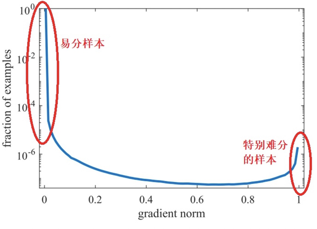
Therefore, the starting point of GHM is: do not focus on easy-to-learn samples, nor on those particularly difficult-to-classify outliers. To this end, the authors defined gradient density, which physically represents the number of samples in the unit gradient magnitude g portion. The final GHM Loss is:

• Dice Loss:

• Similar to Focal Loss, during training, it pushes the model to focus more on difficult samples, using as the weight for each sample. The improved DSC is:
• Mainly proposed to resolve the inconsistency between training and testing F1 metrics, an adaptive loss based on Dice Loss—DSC, is more robust for the F1 metric:

• Adjusting weights for logits: Essentially incorporating category probabilities into the loss and adjusting weights for logits, which is fundamentally a method to alleviate category imbalance through mutual information concepts:

Q7: In the BERT Era, How to Handle Long Text Classification?

Due to memory usage and computational constraints, the input of pre-trained language models like BERT is generally limited to a maximum of 512 tokens. In some scenarios, BERT may perform worse than CNN in handling long text classification. To make BERT more suitable for long text processing, I provide some methods that can be attempted from the perspectives of text processing and improved attention mechanisms:

(1) Text Processing

• Fixed truncation: Generally, information at the beginning and end of the text is more significant; text can be truncated according to a certain proportion from the beginning and end.
• Random truncation: If fixed truncation results in significant information loss, truncation can be performed with different random probabilities in the DataLoader each time; this truncation allows the model to see more variations of cases.
• Truncation & sliding window + prediction averaging: By randomly truncating or using a fixed sliding window to split one sample into multiple samples, the results of multiple samples can be averaged during prediction.
• Truncation + keyword extraction: Direct truncation may lead to information loss; keyword extraction can supplement information. For example: [CLS][truncated text][SEP][keyword1][SEP][keyword2]…

(2) Improved Attention Mechanisms

The attention mechanism used in Transformers has a time complexity of , where is the text length. Recently, some papers have focused on improving the attention mechanism to reduce computational complexity, making it more suitable for handling long text sequences. The main methods include:

• Reformer^[6]: Mainly adopts a locality-sensitive hashing mechanism (LSH), which is similar to bucket sorting: grouping similar vectors first and only calculating the dot product between similar vectors, reducing time complexity to O(nlog(n)); considering that similar vectors may be placed in different buckets, Reformer performs multiple rounds of LSH, but this may reduce efficiency.
• Linformer^[7]: Proposes that self-attention is low-rank, with information concentrated in a small number of (k) maximum singular values. Linformer uses linear mapping to reduce time complexity to , where k is close to linear time. However, practical results indicate that increasing k yields better results, generally set to 256 or 512.
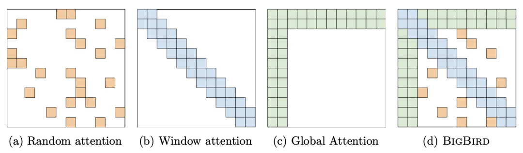
• Longformer^[8]: Adopts a sliding window mechanism, calculating local attention only within a fixed window size w, reducing complexity to , where it approaches linear time (still typically set to 512 in practice); to expand the receptive field, a “dilated sliding window mechanism” can also be used; global attention can also be calculated locally at special positions, such as at [CLS]. For more details, refer to “Longformer: The Transformer for Long Documents”.
• Big Bird^[9]: Builds on Longformer by adding random attention; currently the SOTA for long sequence modeling, refreshing SOTA for QA and summarization, and proving to be Turing complete. As shown in the figure below:

For most long text classification problems, I recommend prioritizing the “text processing” approach. For those with conditions, the aforementioned “improved attention mechanisms” can be attempted, such as continuing to pre-train the already pre-trained RoBERTa using the Longformer mechanism. Longformer has been open-sourced and can be optimized and accelerated directly on CUDA kernels.

Q8: Pre-training Fusion: A Weapon for NLP Competitions!

In major NLP competitions, model fusion (ensemble) is an important tool for boosting scores, and beyond the fusion of different models, another more effective method is—pre-training fusion.

In NLP tasks, the differences in predictions between different models depend more on the underlying models (embedding layer) than in the CV field, where it often depends on the heterogeneity of the upper models.

So how can we enrich the underlying models? A direct way is to fuse different pre-trained models: for example, one can unify word2vec, elmo, BERT, XLNET, ALBERT as feature extractors, but attention should be paid to the following (some content is referenced from “Teacher Wang Ran’s Course”^[10], which I have summarized and integrated):

• Generally, fine-tuning is not necessary. Of course, one can first fine-tune BERT, XLNET, and ALBERT individually and then integrate the features.
• The tokenizer can use the tokenizer of the best pre-trained model or simultaneously use the tokenizers of different pre-trained models.
• Do not overlook the importance of simple word vectors. Supplementing with character/word vectors and bi-gram vectors is crucial for enriching the underlying models.
• When configuring the upper model, pay attention to adjusting the learning rates. Feeding the integrated underlying features into biLSTM or CNN can also concatenate biLSTM and CNN as the upper model. During training, one can first freeze the underlying pre-trained models and only adjust the learning rate of the upper model (larger), and finally adjust the global learning rate (smaller).
• Lastly, the CLS must be used again. Regardless of how the upper model is structured, the CLS feature should directly enter the fully connected layer.

Q9: Have You Seriously Constructed an Offline Test Set? High Indicators May Be Inflated!

Often when we construct a test set, we automatically divide the test set based on the initial labeled set, which is perfectly fine in the early stages of the task. However, we cannot trust high indicators and assume everything is fine. The evaluation phase of the model is crucial; we cannot wait until it is online to realize this, nor can we always wait for online bad cases to iterate.

The best paper at ACL 2020, “Beyond Accuracy: Behavioral Testing of NLP Models with CHECKLIST”, tells us to evaluate multiple “abilities” of the model through CheckList, which can quickly generate a large number of test samples.

In practice, I have found that to make evaluations more comprehensive, we can:

1. Accumulate a synonym library, obscure characters, conduct nature-invariant tests, and vocabulary tests;
2. Construct adversarial samples for attack testing;
3. Prevent problems before they occur by pre-collecting data to find high-uncertainty cases for testing;

Discovering bugs from the above tests is naturally a good thing; exposing problems gives us confidence.

The recently open-sourced OpenAttack text adversarial attack toolkit can also help us with robustness testing, including text preprocessing, victim model access, adversarial sample generation, adversarial attack evaluation, and adversarial training. Adversarial attacks can help expose the weaknesses of victim models, improving model robustness and interpretability, which has significant research significance and application value.

Q10: When Updating and Iterating Models, How to Conduct Incremental Learning Without Forgetting Previous Memories?

During the updating and iteration of modeling methods, there may be a forgetting issue, where previously processed cases no longer work. If there are not many bad cases, rule optimization is relatively robust, and a bypass can be set with rules specifically to handle emergency bad cases.

Additionally, I provide the following solutions to this problem:

1. Directly mix existing data with original data for training;
2. Freeze the feature extraction layer and only update the softMax fully connected layer for new categories;
3. Use knowledge distillation methods. When training with a mix of existing and original data, distill the original categories to guide the new model’s learning.
4. Unify classification labels into label embedding; newly added categories can be constructed separately without affecting original categories, transforming classification into a matching and ranking problem.

Q11: In Low Time Consumption Scenarios, How to Make TextCNN Approach BERT’s Performance?

While BERT is powerful, deploying a classification model directly using BERT in low time consumption and low machine scenarios is usually unfeasible. Can we use a lightweight model like TextCNN to approach BERT’s performance?

To address this issue, we typically employ knowledge distillation techniques. The essence of distillation is function approximation, but if we directly distill BERT (Teacher model) into a very lightweight TextCNN (Student model), the indicators generally decline.

How can we mitigate this situation? I provide two distillation schemes based on the size of the unlabeled data—model distillation and data distillation.

(1) Model Distillation

If the unlabeled data in the business is scarce, we typically use logits approximation (value approximation) for TextCNN learning, which can be termed model distillation. This is an offline distillation method: first fine-tune the Teacher model, then freeze it, and allow the Student model to learn. To avoid a noticeable decline in indicators after distillation, we can improve it in the following ways:

• Data augmentation: Introduce text augmentation techniques during distillation; specific augmentation techniques can be referenced in “Exploring the Dilemma of Few Samples in NLP”. TinyBERT employs augmentation techniques to assist distillation.
• Ensemble distillation: Integrate logits from different Teacher models (such as different pre-trained models) for TextCNN learning. Ensemble distillation + data augmentation can effectively prevent significant declines in indicators.
• Joint distillation: Unlike offline distillation, this is a joint training method. While training the Teacher model, the logits are simultaneously passed to the Student model for learning. Joint distillation can reduce the gap between highly heterogeneous Teacher and Student models, allowing the Student model to gradually learn from an intermediate state and better mimic Teacher behavior.

(2) Data Distillation

If the business has a large amount of unlabeled data, we can use label approximation for TextCNN learning. This method is called data distillation. Its essence is similar to pseudo-labeling methods: allowing the Teacher model to pseudo-label unlabeled data and then letting the Student model learn. The specific steps are:

1. Training 1: Fine-tune BERT on labeled dataset A to train a bert_model;
2. Pseudo-label: The bert_model predicts a large amount of unlabeled data U (pseudo-label), and then scores based on confidence, selecting high-confidence data B to fill into labeled data A, transforming the labeled data into (A+B);
3. Training 2: Train TextCNN based on labeled data A+B to obtain textcnn_model_1;
4. Training 3 (optional): Re-train the textcnn_model_1 based on labeled data A to form the final model textcnn_model_2;

For the above two distillation methods, I conducted experiments on a business task with 21 categories (100 samples per category), and the related results are as follows:

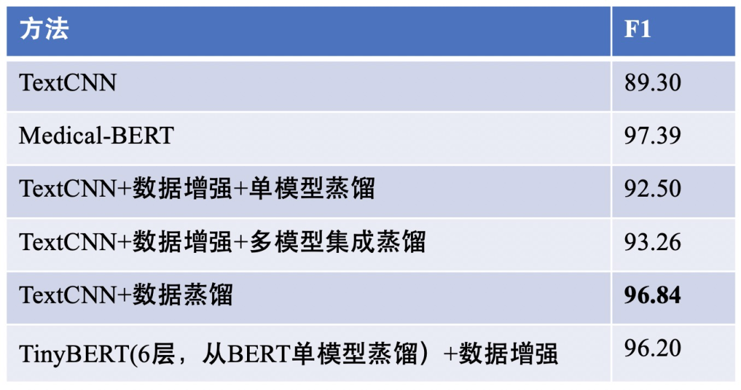
As shown in the figure, if we can obtain more unlabeled data, using data distillation can be more effective, allowing a lightweight TextCNN to approach BERT as closely as possible.

However, some readers may ask why not directly distill into a shallow BERT? This is certainly possible, but the reason I recommend TextCNN here is: it is very lightweight and allows for easier incorporation of business-related features (which will be detailed in a subsequent article).

If you still want to distill into a shallow BERT, we need to consider the gap between the domain we are in and the original pre-training domain of BERT. If the gap is large, we should not stop pre-training; continue domain pre-training and then distill; or pre-train a shallow BERT from scratch. Additionally, when deploying BERT, we can also perform operator fusion (Faster Transformer) or mixed precision methods.

In Conclusion

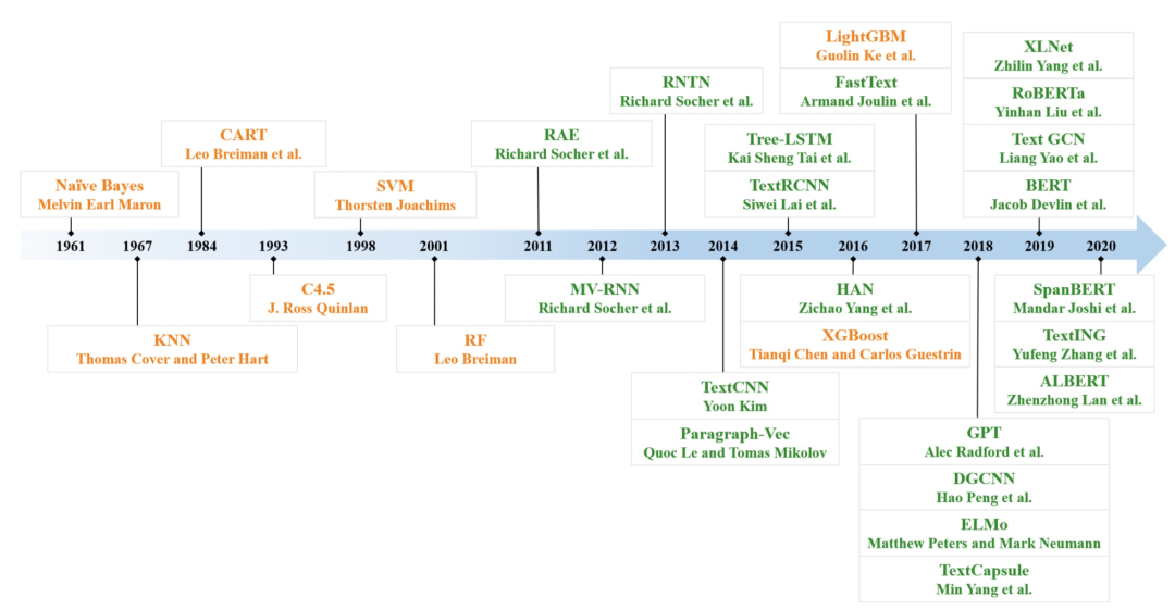
Let us pay tribute to those classification models that accompanied us into the world of NLP~

Download 1: Hands-on Learning Deep Learning
Reply "Hands-on Learning" in the backend of the Machine Learning Algorithms and Natural Language Processing public account to obtain the 547-page electronic book and source code of "Hands-on Learning Deep Learning".
This book covers both the methods and practices of deep learning, explaining the technologies and applications of deep learning from a mathematical perspective, and includes runnable code to show readers how to solve problems in practice.

Download 2: Repository Address Sharing
Reply "Code" in the backend of the Machine Learning Algorithms and Natural Language Processing public account to obtain 195 papers from NAACL + 295 papers from ACL 2019 with open-source code. The open-source address is as follows: https://github.com/yizhen20133868/NLP-Conferences-Code

Heavyweight! The Machine Learning Algorithms and Natural Language Processing exchange group has officially been established! There are abundant resources in the group, and everyone is welcome to join for learning!

Extra bonus resources! Qiu Xipeng's deep learning and neural networks, PyTorch official Chinese tutorial, data analysis using Python, machine learning study notes, Chinese version of pandas official documentation, effective java (Chinese version), and 20 other welfare resources.

How to get: After entering the group, click on the group announcement to get the download link.
Note: Please modify the remark when adding as [School/Company + Name + Direction]. For example, --- Harbin Institute of Technology + Zhang San + Dialogue System.
The account owner, please avoid business matters. Thank you!

Recommended Reading:
A Review of Open-Domain Knowledge Base Question Answering Research
Automatically Train Your Deep Neural Networks Using PyTorch Lightning
Collection of Common Code Snippets in PyTorch

References

[1] xDeepFM: Combining Explicit and Implicit Feature Interactions for Recommender Systems: https://arxiv.org/pdf/1803.05170.pdf[2] Description Based Text Classification with Reinforcement Learning: https://arxiv.org/pdf/2002.03067.pdf[3] Decoupling Representation and Classifier for Long-Tailed Recognition: https://arxiv.org/pdf/1910.09217.pdf[4] Dynamic Curriculum Learning for Imbalanced Data Classification: https://arxiv.org/pdf/1901.06783.pdf[5] https://zhuanlan.zhihu.com/p/80594704[6] REFORMER: THE EFFICIENT TRANSFORMER: https://arxiv.org/pdf/2001.04451.pdf[7] Linformer: Self-Attention with Linear Complexity: https://arxiv.org/pdf/2006.04768.pdf[8] Longformer: The Long-Document Transformer: https://arxiv.org/pdf/2004.05150.pdf[9] Big Bird: Transformers for Longer Sequences: https://arxiv.org/pdf/2007.14062.pdf[10] Teacher Wang Ran’s Course: https://time.geekbang.org/course/intro/100046401