Click the above “Beginner’s Visual Learning“, select to add “Star” or “Top“
Important content delivered promptly
Introduction
Convolutional Neural Networks (CNN) are a class of feedforward neural networks with deep structures that include convolutional computations, representing one of the key algorithms of deep learning. The classic neural network structures are LeNet-5, AlexNet, and VGGNet. This article explains classic convolutional neural networks.
This article is sourced from the notes of Professor Andrew Ng’s Deep Learning Course[1].
Author: Huang Haiguang[2]
Note: The notes and assignments (including data, original assignment files), and videos can be downloaded from GitHub[3].
The Main Text Begins
Classic Networks
Let’s learn about several classic neural network structures, specifically LeNet-5, AlexNet, and VGGNet. Let’s get started.
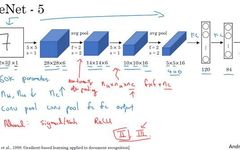
First, let’s take a look at the structure of LeNet-5. Assume you have a 32×32×1 image, LeNet-5 can recognize handwritten digits in the image, such as the handwritten digit 7. LeNet-5 is trained on grayscale images, so the image size is only 32×32×1. In fact, the structure of LeNet-5 is very similar to the last example we discussed last week, using 6 filters of size 5×5 with a stride of 1. Since 6 filters are used with a stride of 1 and padding of 0, the output is 28×28×6, reducing the image size from 32×32 to 28×28. Then we perform a pooling operation; in the era when this paper was written, people preferred average pooling, while nowadays we might use max pooling more often. In this example, we perform average pooling with a filter width of 2 and a stride of 2, which reduces the height and width of the image by half, resulting in an output image of 14×14×6. I think this image is not drawn to scale; if drawn to scale, the new image size should be exactly half of the original image.
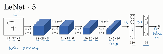
Next is the convolutional layer, where we use a set of 16 filters of size 5×5, resulting in a new output with 16 channels. The paper on LeNet-5 was written in 1998, at a time when people did not use padding, or always used valid convolution, which is why the height and width of the image shrink with each convolution, reducing this image from 14×14 to 10×10. Then we have another pooling layer, halving the height and width again, resulting in a 5×5×16 image. Multiplying all the numbers gives a product of 400.
The next layer is the fully connected layer, which has 400 nodes, each with 120 neurons, creating one fully connected layer. However, sometimes a portion of these 400 nodes is extracted to form another fully connected layer, resulting in 2 fully connected layers.
The final step is to use these 84 features to obtain the final output. We can also add one more node here to predict the value, with 10 possible values corresponding to recognizing the digits 0-9. In the current version, the softmax function is used to output ten classification results, whereas at that time, the LeNet-5 network used another classifier at the output layer, which is rarely used today.
Compared to modern versions, this neural network is smaller, with only about 60,000 parameters. Nowadays, we often see neural networks with 10 million to 100 million parameters, and networks 1000 times larger are not uncommon.
Nevertheless, if we look from left to right, we can see that as the network becomes deeper, the height and width of the image shrink, from the initial 32×32 to 28×28, then to 14×14, 10×10, and finally down to 5×5. At the same time, as the network depth increases, the number of channels keeps increasing, from 1 to 6, then to 16.
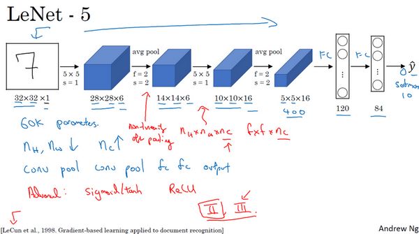
This neural network also follows a pattern that is still frequently used today, which is one or more convolutional layers followed by a pooling layer, followed by several convolutional layers and another pooling layer, then a fully connected layer, and finally the output. This arrangement is quite common.
For those who wish to attempt reading the papers, I will add a few points. The next section is primarily for those planning to read classic papers, so it will be more in-depth. You can completely skip this content as it serves as a review of the history of neural networks, and it’s okay if you don’t understand it.
When you read this classic paper, you will find that in the past, people used the sigmoid function and the tanh function instead of the ReLu function. The sigmoid function and tanh function are precisely what this paper uses. The uniqueness of this network structure also lies in the relationships between the layers, which seems quite interesting today.
For example, if you have a network with channels, using filters of size , each filter’s channel number is the same as that of the previous layer. This is because, at that time, the speed of computers was very slow, and to reduce computation and parameters, the classic LeNet-5 network used a very complex computation method, with each filter utilizing the same number of channels as the input module. These complex details mentioned in the paper are generally not used today.
I believe the final step taken back then has not really been completed even now, which is that the classic LeNet-5 network performed non-linear function processing after pooling. In this example, the sigmoid function was used after the pooling layer. If you really read this paper, this will be one of the most difficult parts to understand, and we will discuss it in future courses.
The next network structure to be discussed is simpler; most of the content in the slides comes from the second and third paragraphs of the original text, while the latter paragraphs introduce another idea. The deformable network mentioned in the text has not gained widespread application today, so when reading this paper, I suggest focusing on the second paragraph, which emphasizes this network structure, and skimming the third paragraph, which mainly presents some interesting experimental results.
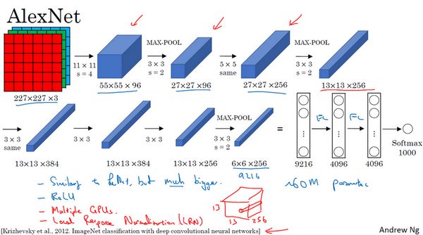
The second type of neural network I want to illustrate is AlexNet, named after the first author Alex Krizhevsky, with co-authors ilya Sutskever and Geoffery Hinton.
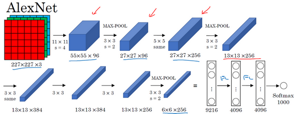
AlexNet first uses an image of size 227×227×3 as input. In fact, the image used in the original text is 224×224×3, but if you try to derive it, you will find that the size of 227×227 is better. In the first layer, we use 96 filters of size 11×11 with a stride of 4; since the stride is 4, the size reduces to 55×55, approximately a 4-fold reduction. Then, a 3×3 filter is used to construct a max pooling layer, with a stride of 2, reducing the convolutional layer size to 27×27×96. Next, we perform a 5×5 convolution, and after padding, the output is 27×27×276. Then we perform max pooling again, reducing the size to 13×13. Another same convolution is performed with the same padding, yielding a result of 13×13×384 with 384 filters. Another same convolution is performed in the same manner. After another max pooling, the size reduces to 6×6×256. The result of 6×6×256 equals 9216, which is flattened into 9216 units, followed by some fully connected layers. Finally, the softmax function is used to output the identification results, determining which of the 1000 possible objects it corresponds to.
In fact, this neural network shares many similarities with LeNet, but AlexNet is much larger. As mentioned earlier, LeNet or LeNet-5 has about 60,000 parameters, while AlexNet contains about 60 million parameters. When training images and datasets, AlexNet can handle very similar basic structural modules, which often contain a large number of hidden units or data, and this is where AlexNet excels. Another reason AlexNet performs better than LeNet is that it uses the ReLu activation function.
Similarly, I will also discuss some more profound content, but if you do not plan to read the papers, you can skip it. The first point is that when this paper was written, the processing speed of GPU was still relatively slow, so AlexNet adopted a very complex method to train on two GPUs. The basic principle is that these layers are split across two different GPUs, and there is a specific method for communication between the two GPUs.
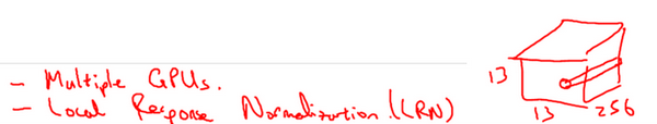
The paper also mentions that the classic AlexNet structure includes another type of layer called the “Local Response Normalization layer” (LRN layer), which is not commonly applied, so I did not specifically discuss it. The basic idea of local response normalization is that if this is a section of the network, say 13×13×256, the LRN needs to select a position, such as this one, and through this position across the entire channel, it can obtain 256 numbers and normalize them. The motivation for performing local response normalization is that for each position in this 13×13 image, we might not need too many highly activated neurons. However, many researchers later found that LRN does not play a significant role, which should be one of the contents I have crossed out because it is not important, and we do not use LRN to train networks anymore.
If you are interested in the history of deep learning, I believe that before AlexNet, deep learning had already gained some attention in speech recognition and a few other fields, but it was through this paper that the computer vision community began to pay attention to deep learning and became convinced that deep learning could be applied in the field of computer vision. Since then, the influence of deep learning in computer vision and other fields has been increasing day by day. If you do not plan to read papers in this area, you can skip this lesson. However, if you want to understand some related papers, this one is relatively easy to understand and will be easier to learn.
AlexNet network structure appears relatively complex, containing many hyperparameters. These numbers (55×55×96, 27×27×96, 27×27×256, etc.) are all provided by Alex Krizhevsky and his co-authors.
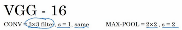
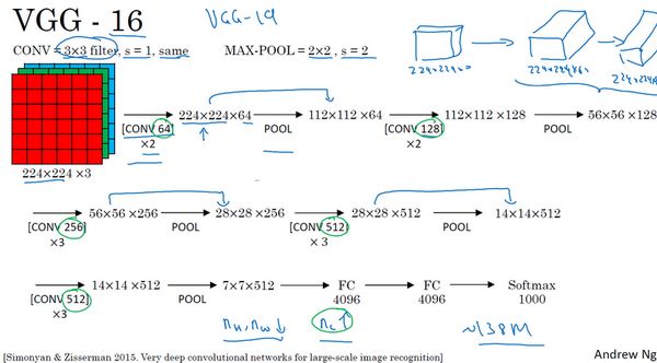
The third and final example to be discussed in this lesson is VGG, also known as VGG-16 network. It is worth noting that the VGG-16 network does not have as many hyperparameters; it is a simple network that focuses solely on constructing convolutional layers. First, we construct convolutional layers using 3×3 filters with a stride of 1, with the padding parameter being same in the convolution. Then, a max pooling layer is constructed using a 2×2 filter with a stride of 2. Therefore, one of the significant advantages of the VGG network is that it indeed simplifies the neural network structure. Let’s discuss this network structure in detail.
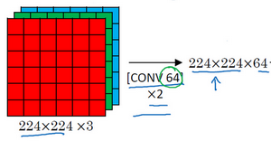
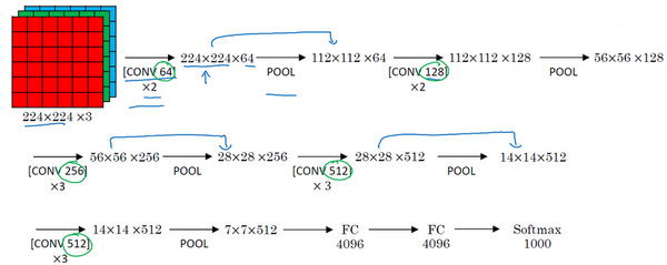
Assuming we want to recognize this image, in the first two layers, we use 64 filters of size 3×3 to convolve the input image, resulting in an output of 224×224×64 because we used same convolution, maintaining the same number of channels. VGG-16 is actually a very deep network, and I have not drawn all the convolutional layers here.
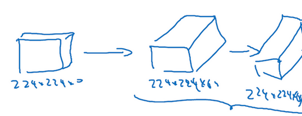
Assuming this small image is our input image, with dimensions of 224×224×3, after the first convolution, we obtain a feature map of 224×224×64, followed by another layer of 224×224×64, resulting in two convolutional layers with a thickness of 64, meaning we convolved with 64 filters twice. As I mentioned earlier, all the filters used here are of size 3×3 with a stride of 1, and all use same convolution, so I won’t draw all the layers again, just using a string of numbers to represent these networks.
Next, we create a pooling layer, which compresses the input image from 224×224×64 to what size? That’s right, reduced to 112×112×64. Then there are several convolutional layers using 129 filters, and some same convolutions, we see what the output is, which is 112×112×128. Then we perform pooling, which can be derived to result in (56×56×128). Next, we use 256 identical filters to perform three convolution operations, then pool, then convolve three more times, and pool again. After several rounds of operations, we obtain the final feature map of 7×7×512, which is then connected to 4096 units, followed by softmax activation to output the recognition result from 1000 objects.
By the way, the number 16 in VGG-16 refers to the 16 convolutional layers and fully connected layers in this network. It is indeed a large network, containing about 138 million parameters, which is still considered a very large network even by today’s standards. However, the structure of VGG-16 is not complex, which is very appealing, and this network structure is very orderly, with several convolutional layers followed by pooling layers that can compress the image size. The pooling layers reduce the height and width of the image, while the number of filters in the convolution layers changes in a certain pattern, doubling from 64 to 128, then to 256 and 512. The authors may have thought that 512 was large enough, so the later layers do not double anymore. In any case, doubling at every step, or doubling the number of filters in each group of convolutional layers, is another simple principle in designing this network structure. This relatively consistent network structure is attractive to researchers, while its main drawback is the enormous number of features required for training.
Some articles also introduce the VGG-19 network, which is even larger than VGG-16. If you want to know more details, please refer to the notes at the bottom of the slides, reading the paper by Karen Simonyan and Andrew Zisserman. Since the performance of VGG-16 is almost on par with VGG-19, many people still choose to use VGG-16. One aspect I particularly like about it is that the paper reveals that as the network deepens, the height and width of the image continuously shrink in a certain pattern, halving after each pooling, while the number of channels keeps increasing, again doubling after each group of convolution operations. In this sense, the paper is very appealing.
That concludes the discussion of three classic network structures. If you are interested in these papers, I recommend starting with the paper introducing AlexNet, then moving on to the VGG paper, and finally the LeNet paper. Although some parts may be obscure, they are very helpful for understanding these network structures.
Good news, the Beginner’s Visual Learning team’s knowledge circle is now open! To thank everyone for their support and love, the team has decided to allow free access to the knowledge circle worth 149 yuan. Everyone should seize the opportunity!

Download 1: OpenCV-Contrib Extension Module Chinese Tutorial Reply to “Beginner’s Visual Learning” in the background of the public account:Chinese Tutorial for Extension Modules, to download the first Chinese version of the OpenCV extension module tutorial available online, covering more than twenty chapters including installation of extension modules, SFM algorithms, stereo vision, object tracking, biological vision, super-resolution processing, etc.Download 2: Python Visual Practical Projects 52 Lectures Reply to “Python Visual Practical Projects” in the background of the public account:, to download 31 visual practical projects including image segmentation, mask detection, lane detection, vehicle counting, eyeliner addition, license plate recognition, character recognition, emotion detection, text content extraction, facial recognition, etc., to help quickly learn computer vision.Download 3: OpenCV Practical Projects 20 Lectures In the background of the public account, reply to: OpenCV Practical Projects 20 Lectures, to download 20 practical projects based on OpenCV to advance your learning of OpenCV.
Discussion Group
Welcome to join the reader group of the public account to exchange ideas with peers. Currently, there are WeChat groups for SLAM, 3D vision, sensors, autonomous driving, computational photography, detection, segmentation, recognition, medical imaging, GAN, algorithm competitions, etc. (which will be gradually subdivided in the future). Please scan the WeChat number below to join the group, and note: “Nickname + School/Company + Research Direction”, for example: “Zhang San + Shanghai Jiao Tong University + Visual SLAM”. Please follow the format for notes, otherwise, entry will not be approved. After successful addition, you will be invited into relevant WeChat groups based on your research direction. Please do not send advertisements in the group; otherwise, you will be removed from the group. Thank you for your understanding~